Accurate and efficient sampling of interpolated functions

Question

Suppose we are given two interpolated functions

f1 = Interpolation[{{0, 0}, {1, 2}, {3, 5}, {4, 2}, {8, -1}}, InterpolationOrder -> 0];
f2 = Interpolation[{{0, 0}, {1, 3}, {3, 7}, {4, 2}, {8, 0}}, InterpolationOrder -> 1];

and one derived function

f3 = FunctionInterpolation[f1[t] - f2[t], {t, 0., 8.}];

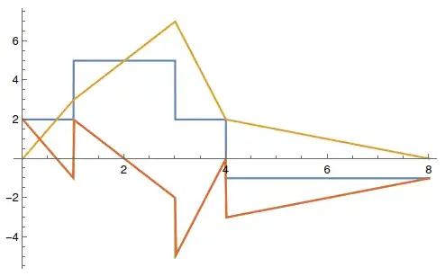
Plotting those functions shows that f3 is not a very accurate representation of the result.

Plot[{f1[t], f2[t], f1[t] - f2[t], f3[t]}, {t, 0, 8}]

This can be improved by defining f3 as follows

f3 = FunctionInterpolation[
       f1[t] - f2[t],
       {t, 0., 8.},
       InterpolationPoints -> 300, 
       InterpolationOrder -> 1
     ];

but at the cost of oversampling.

A simple but rather hacky way to represent f3 more accurately without oversampling is

f3 = Interpolation[
       Cases[Plot[f1[t] - f2[t], {t, 0, 8}], Line[_], Infinity][[1, 1]],
       InterpolationOrder -> 1
     ]

I also tried to construct an InterpolatingFunction from MeshCoordinates@DiscretizeRegion@ImplicitRegion[f1[t] - f2[t] == y, {{t, 0, 8}, {y, -6, 3}}]. However, this does not work out of the box because points are duplicated due to the presence of discontinuities.

How would you approach the problem?

Update: The following use case is one example where accurate and efficient sampling is necessary. Suppose the dependent variable represents a date (AbsoluteTime[DateObject[...]]) and the goal is to construct a TimeSeries object of f1[t] + f2[t] that takes interpolation into account.

Answer 1

First off, @ cvgmt's suggestion f3[t_] := f1[t] - f2[t] seems the easiest and most efficient way to proceed.

Second, here's a way for those who wish to do it anyway: Using discontInterpolation[] from Interpolating data with a step, we get this:

f1 = Interpolation[{{0, 0}, {1, 2}, {3, 5}, {4, 2}, {8, -1}}, 
   InterpolationOrder -> 0];
f2 = Interpolation[{{0, 0}, {1, 3}, {3, 7}, {4, 2}, {8, 0}}, 
   InterpolationOrder -> 1];
grid = Union[f1@"Grid", f2@"Grid"];
dupegrid = Riffle[Most@grid, Rest@grid];
fpieces =
  Subtract @@ {f1@"GetPolynomial"[#, x - #], 
      f2@"GetPolynomial"[#, x - #]} & /@ Rest@grid;
dfpieces = D[fpieces, x];
fvals = MapThread[ReplaceAll,
    {fpieces, Partition[{x -> #} & @@@ grid, 2, 1]}] // Flatten;
dfvals = MapThread[ReplaceAll,
    {dfpieces, Partition[{x -> #} & @@@ grid, 2, 1]}] // Flatten;
f3 = discontInterpolation[Transpose@{dupegrid, fvals, dfvals}];
Plot[{f1[x], f2[x], f3[x]}, {x, 0, 8}]

The two functions f1 and f2 do not have to have the same grid. You need the derivatve values to make the discontinuous interpolation work (AFAIR, an apparent and undocumented requirement of InterpolatingFunction), so you're stuck with a minimum order-3 interpolation; otherwise, it uses a minimal grid and sampling. Since we control the derivatives, the cubic polynomials in the interpolant turn out to have coefficients of zero on the quadratic and cubic terms. So in effect, it's a linear interpolation, just as it appears in the plot.

Manual construction of an InterpolatingFunction is sorta DANGEROUS. SAVE YOUR WORK before you try it. Since there isn't safe access to the full functionality of InterpolatingFunction, there's not much choice. Perhaps someone could get NDSolve[] to construct f1[t] - f2[t].

Answer 2

What about (see @cvgmt's comment)

f3=f1&-f2&