Question on DSolve's IncludeSingularSolutions option. Why some output do not agree with definition?

Question

in V 13.1, DSolve added a very useful option IncludeSingularSolutions which according to Mathematica own documentation says

Singular solutions cannot be obtained by assigning finite numerical values to the arbitrary constants in the general solution for a nonlinear differential equation.

But I see 100's of solutions given that DSolve says they are singular, but can be obtained from the general solution. Here are just 3 examples

DSolve[x^2*(y'[x])^2 - y[x]^2 == 0, y[x], x]
DSolve[x^2*(y'[x])^2 - y[x]^2 == 0, y[x], x,  IncludeSingularSolutions -> True]

The first one is the general solution. But we see that by setting c1 to zero, it gives 0 as the solution. But Mathematica says that y[x] -> 0 is a singular solution.

Here are two more examples.

DSolve[x*(y'[x])^2 - (2*x + 3*y[x])*y'[x] + 6*y[x] == 0, y[x], x]
DSolve[x*(y'[x])^2 - (2*x + 3*y[x])*y'[x] + 6*y[x] == 0, y[x], x,  IncludeSingularSolutions -> True]

DSolve[x^2*(y'[x])^2 - 5*x*y[x]*y'[x] + 6*y[x]^2 == 0, y[x], x]
DSolve[x^2*(y'[x])^2 - 5*x*y[x]*y'[x] + 6*y[x]^2 == 0, y[x], x, IncludeSingularSolutions -> True]

Now here is an example, where the singular solution generated is a true one

  DSolve[y[x]==y'[x]*x+1/y'[x],y[x],x,IncludeSingularSolutions -> True]

Ignoring the Indeterminate one, (that should not show up), we see that {y[x] -> -2 Sqrt[x]}, {y[x] -> 2 Sqrt[x]} are true singular solutions, because no value for the constant of integration will generate these solutions.

I see no possible issues tag in the help page on this command.

my question is: Why DSolve says these are singular solutions when they can be obtained from the general solution?

I was using Mathematica to verify my hand solution when I noticed this.

V 13.2 on windows 10.

Answer 1

I will give it a go with the risk of humiliating myself.

From the documentation there's a worked example; see Properties & Relations. That example explains how to obtain the singular solution(s) from the envelope for the family of curves by the general solution.

In that example we are told that we need to consider the general solution of a nonlinear ODE and to construct the envelope for the family of curves defined by the general solution. After that, we wish to consider the solution and its derivative by setting the latter to zero and eliminate the constant. Solve for y[x] and that gives the output of IncludeSingularSolutions. The worked example in the docs is the following:

Step 1:

DSolve[y[x] == x*y'[x] + y'[x]^2 - 3 y'[x], y[x], x]

which gives

Then, with

sol = y[x] == (y[x] /. %[[1]])

we Eliminate

Eliminate[{sol, D[sol[[2]], C[1]] == 0}, C[1]]

and we solve

Solve[%, y[x]]

We are now at a position to compare to IncludeSingularSolutions -> True

DSolve[y[x] == x*y'[x] + y'[x]^2 - 3 y'[x], y[x], x, 
 IncludeSingularSolutions -> True]

As far as I can tell, but maybe I am missing something(?), we can follow the same steps as the example for case mentioned.

DSolve[y[x] == y'[x]*x + 1/y'[x], y[x], x]
sol = y[x] == (y[x] /. %[[1]])

and then

Eliminate[{sol, D[sol[[2]], C[1]] == 0}, C[1]]
Solve[%, y[x]]

Edit 1: including the other examples mentioned in the OP

The first example

de = DSolve[x^2*(y'[x])^2 - y[x]^2 == 0, y[x], x]
sol1 = y[x] == (y[x] /. de[[1]])
sol2 = y[x] == (y[x] /. de[[2]])

and then

Eliminate[{sol1, D[sol1[[2]], C[1]] == 0}, C[1]]
Eliminate[{sol2, D[sol2[[2]], C[1]] == 0}, C[1]]

and we got the y[x]->0 solution.

Edit 2: the second example from the OP

de = DSolve[x*(y'[x])^2 - (2*x + 3*y[x])*y'[x] + 6*y[x] == 0, y[x], 
  x]
sol1 = y[x] == (y[x] /. de[[1]])
sol2 = y[x] == (y[x] /. de[[2]])

Eliminate[{sol1, D[sol1[[2]], C[1]] == 0}, C[1]]
Eliminate[{sol2, D[sol2[[2]], C[1]] == 0}, C[1]]

Edit 3: the third example

de = DSolve[x^2*(y'[x])^2 - 5*x*y[x]*y'[x] + 6*y[x]^2 == 0, y[x], x]
sol1 = y[x] == (y[x] /. de[[1]])
sol2 = y[x] == (y[x] /. de[[2]])

Eliminate[{sol1, D[sol1[[2]], C[1]] == 0}, C[1]]
Eliminate[{sol2, D[sol2[[2]], C[1]] == 0}, C[1]]

Answer 2

Here's how I approach singular solutions. I sometimes have to think about a step somewhere in the middle, so it's not quite an algorithm yet. I think of an ODE $F(x,y(x),y'(x))=0$ as a manifold $F(x,y,p)=0$ in 3-space on which there is a vector field, called the contact field, corresponding to $p=dy/dx$: The "slope" of a solution curve as viewed from above is given by the height $p$ of the surface. (The solution or integral curve is the parametric curve $(x,y,p)=(x,y(x),y'(x))$.)

There are two sorts of singularities: Those in the manifold itself (such as self-intersections), and those where the field is undefined, which happens when $\partial F/\partial p = 0$.

DSolve also adds solutions, under IncludeSingularSolutions, that are limits of the general solution at boundaries of the domain of the integration parameter (usually C[1]). In fact it seems to check only infinity and zero and does not look into whether there are other boundaries in the domain of C[1].

Since we're looking at examples of DSolve, we can construct mesh functions that show the solution curves on the ODE manifold, which I wanted to share.

Example 1

ode = x^2*(y'[x])^2 - y[x]^2 == 0;
manifold = ode /. {y'[x] -> p, y[x] -> y};
Reduce[{manifold, D[manifold, p]}, {x, y, p}] (* sing sols *)
dsol = DSolve[ode, y, x, IncludeSingularSolutions -> True]
(*ode/.dsol//Simplify*) (* check dsol *)
{mfns, mesh} = dsol // solToMeshFunction // Transpose
ContourPlot3D[manifold // Evaluate,
 {x, -1, 1}, {y, -1, 1.01}, {p, -5.01, 5},
 AxesLabel -> Automatic,
 MeshFunctions -> mfns // Evaluate,
 Mesh -> mesh /. Automatic -> 15 // Evaluate,
 MeshShading -> RandomColor[RGBColor[_, _, _, 0.5], {4, 4, 2}]]

(*
 * A sing. pt. (not sol.) and sing. sol. y == 0
(x == 0 && y == 0) || (y == 0 && p == 0)
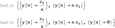
{{y -> Function[{x}, C[1]/x]},
 {y -> Function[{x}, x C[1]]},
 {y -> Function[{x}, 0]}}
{{Function[{x, y, p}, -p x^2], Function[{x, y, p}, p], 
  Function[{x, y, p}, p - 0]}, (* redundent b/c sol is redundant )
 {Automatic, Automatic, {0}}}
)

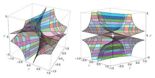
The tartan grid is formed by the two families of solutions, the hyperbolas and lines. The line y == 0 is a singular locus of the manifold that happens to be a solution to the ODE, as well as a particular value of the general solution.

Example 2

ode = x*(y'[x])^2 - (2*x + 3*y[x])*y'[x] + 6*y[x] == 0;
manifold = ode /. {y'[x] -> p, y[x] -> y};
Reduce[{manifold, D[manifold, p]}, {x, y, p}] (* sing sols *)
dsol = DSolve[ode, y, x, IncludeSingularSolutions -> True]
(*ode/.dsol//Simplify*)
{mfns, mesh} = dsol // solToMeshFunction // Transpose
ContourPlot3D[manifold // Evaluate,
 {x, -1, 1}, {y, -1, 1.01}, {p, -3.01, 7},
 AxesLabel -> Automatic,
 MeshFunctions -> mfns // Evaluate,
 Mesh -> mesh /. Automatic -> 15 // Evaluate,
 MeshShading -> RandomColor[RGBColor[_, _, _, 0.5], {4, 4, 2}],
 ViewPoint -> {20, 0, 0}, ViewVertical -> {0, 0, 1}]

(*
 * A sing. pt. (not a sol.) and sing. locus (not a sol.)
(x == 0 && y == 0) ||
 (y == (2 x)/3 && p == 2) || (* y == 2x/3 is split into two cases *)
 (y == (2 x)/3 && x != 0 && p == 2)
{{y -> Function[{x}, x^3 C[1]]},
 {y -> Function[{x}, 2 x + C[1]]},
 {y -> Function[{x}, 0]}}  (* spurious *)
{{Function[{x, y, p}, p/(3 x^2)], Function[{x, y, p}, -2 x + y], 
  Function[{x, y, p}, p - 0]}, {Automatic, Automatic, {0}}}
*)

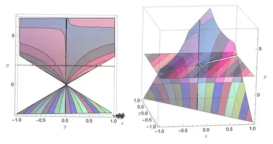
The line y == 0 is not a singular locus of the manifold, just the point at the origin. It happens to be a solution to the ODE, in fact a particular value of the general solution, and perhaps that's why it was retained in the output of DSolve[]. As can be seen, y == 2x/3, which shows up in Reduce[] output, is a self-intersection of the manifold. It is at a height of p == 2 and would have to have slope 2 to be a solution. So it's not a singular solution.

Example 3

This is a classic Clairaut equation.

ode = y[x] == y'[x]*x + 1/y'[x];
manifold = ode /. {y'[x] -> p, y[x] -> y};
Reduce[{manifold, D[manifold, p]}, {x, y, p}] (* sing sols *)
dsol = Cases[DSolve[ode, y, x, IncludeSingularSolutions -> True], 
  s_ /; FreeQ[s, Indeterminate]]
(*ode/.dsol//Simplify*)
{mfns, mesh} = dsol // solToMeshFunction // Transpose
Show[
 ContourPlot3D[p y == 1 + p^2 x, {x, -5, 5.01},
  {y, -5, 5.007}, {p, -10.01, 10},
  AxesLabel -> Automatic, MaxRecursion -> 3, 
  PlotPoints -> {15, 45, 45},
  MeshFunctions -> mfns // Evaluate,
  Mesh -> mesh /. Automatic -> 
     Subdivide[-(9.5^(1/3)), (9.5^(1/3)), 25]^3 // 
   Evaluate,
  MeshShading -> RandomColor[RGBColor[_, _, _, 0.5], {4, 2, 2}]]]

(*
 * Two singular solutions (or one if y^2 == 4x)
(y == -2 Sqrt[x] || y == 2 Sqrt[x]) && x != 0 && p == y/(2 x)
{{y -> Function[{x}, 1/C[1] + x C[1]]},
 {y -> Function[{x}, -2 Sqrt[x]]},
 {y -> Function[{x}, 2 Sqrt[x]]}}
{{Function[{x, y, p}, p], 
  Function[{x, y, p}, p - -(1/Sqrt[Max[1.*10^-16, x]])], 
  Function[{x, y, p}, 
   p - 1/Sqrt[Max[1.*10^-16, x]]]}, {Automatic, {0}, {0}}}
*)

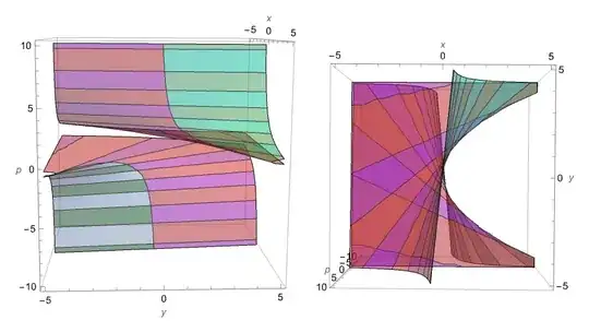
The top view shows that the tangent planes are vertical along the singular solutions. This is equivalent to $\partial F/\partial p = 0$. See DSolve misses a solution of a differential equation for a more in-depth analysis of a similar singular solution.

solToMeshFunctions

solToMeshFunction // ClearAll;
solToMeshFunction::dim = "Dimension of solution ``, expected 1.";
solToMeshFunction::fo = "First-order ODEs only (no systems).";
solToMeshFunction[sols_ : {__List}] := 
  Flatten[solToMeshFunction /@ sols, 1];
solToMeshFunction[{sol_Rule}] := solToMeshFunction[sol];
solToMeshFunction[{_Rule, __Rule}] := Null /; (
    Message[solToMeshFunction::fo]; False);
solToMeshFunction[sol : (y_[x_] -> _)] := 
  solToMeshFunction[DSolve`DSolveToPureFunction[sol]];
solToMeshFunction[sol : (y_ -> Verbatim[Function][{x_}, s_])] /; 
   FreeQ[sol, _C] :=
  With[{yp = y'[x] /. sol /. 
      Power[b_, r_] /; EvenQ[Denominator@r] :> 
       Power[Max[10.^-16, b], r]},
   {{Function @@ Hold[{x, y, p}, p - yp], {0}}}
   ];
solToMeshFunction[sol : (y_ -> Verbatim[Function][{x_}, s_])] :=
  With[{param = DeleteDuplicates@Cases[s, _C, Infinity]},
   If[Length@param != 1,
    Message[solToMeshFunction::dim, Length@param]
    ];
   With[{mf = First@param /. Replace[
          Solve[p == (y'[x] /. sol), param],
          {} :> Solve[y == s, param]
          ] /. 
        Power[b_, r_] /; EvenQ[Denominator@r] :> 
         Power[Max[10.^-16, b], r]},
     {Function @@ Hold[{x, y, p}, #], Automatic} & /@ mf
     ] /; Length@param == 1
   ];