Euler's Method from Python to Mathematica

Question

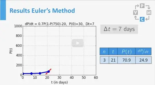
The initial value problem is : $$P'(t)=0.7P(t)(1-\frac{P(t)}{750})-20, P(0)=30$$

The time step is set to $Δt=7$ days

For the algorithm we have:

$f(t,P)=0.7P(1-\frac{P}{750})-20$

with step $h=7$

$t_0=0$.

Euler's method reads in this case $$ P_0 = 30, \quad P_{i+1} = P_i + h \left( 0.7 P_i \left(1- \frac{P_i}{750}\right) -20\right) $$.

My target is to create a table and a plot that will change every time I will the step $Δt$

I have used the following commands

p'[t] == 7/10 p[t]*(1 - p[t]/750) - 20;
p[0]==30
h==7
[![NDSolve\[{p'\[t\] == 7/10 p\[t\]*(1 - p\[t\]/750) - 20, p\[0\]==30}, p\[t\], {t, 0, 1},
 Method -> "ExplicitEuler", "StartingStepSize" -> 7\]][1]][1]

My target is to create a table and a plot that will change every time I will the step $Δt$ and shows $P(T)$ as in the picture below. Is it possible?

Edit:

My professor shared with me the following Python code. However, I am not used to using Python, and I would like to run it in Mathematica. Is it possible? Could anyone help me?

# Program      : Euler's method
# Author       : MOOC team Mathematical Modelling Basics
# Created      : April, 2017
import numpy as np
import matplotlib.pyplot as plt
print("Solution for dP/dt = 0.7*P") # in Python 2.7: use no brackets
Initializations
Dt = 0.1                                # timestep Delta t
P_init = 10                             # initial population 
t_init = 0                              # initial time
t_end = 5                               # stopping time
n_steps = int(round((t_end-t_init)/Dt)) # total number of timesteps
t_arr = np.zeros(n_steps + 1)           # create an array of zeros for t
P_arr = np.zeros(n_steps + 1)           # create an array of zeros for P
t_arr[0] = t_init                       # add the initial P to the array
P_arr[0] = P_init                       # add the initial t to the array
Euler's method
for i in range (1, n_steps + 1):
    P = P_arr[i-1]
    t = t_arr[i-1]
    dPdt = 0.7P                        # calculate the derivative 
    P_arr[i] = P + DtdPdt              # calculate P on the next time step
    t_arr[i] = t + Dt                   # adding the new t-value to the list
Plot the results
fig = plt.figure()                      # create figure
plt.plot(t_arr, P_arr, linewidth = 4)   # plot population vs. time
plt.title('dP/dt = 0.7P, P(0)=10', fontsize = 25)

plt.xlabel('t (in days)', fontsize = 20)
plt.ylabel('P(t)', fontsize = 20)
plt.xticks(fontsize = 15)
plt.yticks(fontsize = 15)
plt.grid(True)                          # show grid 
plt.axis([0, 5, 0, 200])                # define the axes
plt.show()                              # show the plot
save the figure as .jpgde
```

Answer 1

ode = p'[t] == 7/10 p[t]*(1 - p[t]/750) - 20;
ic = p[0] == 30
sol = p /. First@NDSolve[{ode, ic}, p, {t, 0, 1}, Method -> "ExplicitEuler", StartingStepSize" -> 7];
exact = p[t] /. First@DSolve[{ode, ic}, p[t], t]
sol["Methods"]

The above gives you all properties of the numerical solution. You can access the data used and compare to exact solution as follows

y = sol["ValuesOnGrid"] // Chop
x = First@sol["Coordinates"]
data = Transpose[{x, y}];
p1 = ListPlot[data, PlotStyle -> Red, GridLines -> Automatic, GridLinesStyle -> LightGray];
p2 = Plot[exact, {t, 0, 1}, PlotStyle -> Blue];
Show[p1, p2, PlotLabel -> "Exact vs. Euler"]

Euler method gets worst with time. You can see this if you change t to 10 seconds instead of 1

Answer 2

MaxStepFraction is needed if you want fewer than ten steps.

Manipulate[
 With[{sol = Quiet[
     NDSolveValue[{p'[t] == 7/10 p[t]*(1 - p[t]/750) - 20, 
       p[0] == 30}, p, {t, 0, n*h}, 
      Method -> {"FixedStep", Method -> "ExplicitEuler"}, 
      StartingStepSize -> h, MaxStepFraction -> 1, MaxSteps -> n],
     NDSolveValue::mxst]},
  foo = sol;
  Grid[{{Style["Results Euler's Method", 
      "Subsubsection"]}, {ListLinePlot[sol, Mesh -> All, 
      PlotRange -> {{0, 60}, {-10, 1000}}],
     Column[{
       Row[{"\[CapitalDelta]t = ", h, " days"}],
       "",
       Grid[{{"n", "t", HoldForm[P[t]], HoldForm[P'[t]]},
         {n, n*h, sol[n*h], sol'[n*h]}},
        Dividers -> All]
       }]}
    }]
  ],
 {{h, 7, "\[CapitalDelta]t"}, 1., 15},
 {{n, 3, "steps"}, 1, 60, 1}
 ]