How can we apply specific boundary conditions with NDEigensystem?

Question

I'm solving an eigenvalue problem with special b.c. mentioned in the paper Edge states in gated bilayer-monolayer graphene ribbons and bilayer domain walls. (See Eq.(3)(6)(7) and the paragraph after (9). ) The paper author claims the problem is solved with COMSOL MULTIPHYSICS. I tried with NDEigensystem but failed.

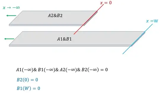
The system involves four coupled ODE [$A1(x),B1(x),A2(x),B2(x)$] defined in the interval $x=\{-\infty,0\}$ and 2 ODE [$A(x),B(x)$] Eqs for $x=\{0,W\}$, The b.c.s are:

$A1(0)=A(0)$
$B1(0)=B(0)$
$B2(0)=0$
$B(W)=0$

and all functions $(A1,B1,A2,B2)$ in the left interval go to zero as $x$ goes to $-\infty$. Here is my trivial try

systm1[k_]:=Module[{a=400,hv = 0.65875 10^3, W = 23.86},{vals,funs}=NDEigensystem[{
hv(-B1'[x]-k B1[x]) +50 A1[x],
hv(A1'[x]-k A1[x]) +50 B1[x]+a A2[x],
hv(B2'[x]+k B2[x]) -50 A2[x]+a B1[x],
hv(-A2'[x]+k A2[x]) -50 B2[x],
hv(-B'[x]-k B[x])+50A[x] ,
hv(A'[x]-k A[x])+50B[x] ,
DirichletCondition[{A1[0]==A[0],B1[0]==B[0],B2[0]==0,B[W]==0},True]},{A1[x],B1[x],A2[x],B2[x],A[x],B[x]},{x,-10W,10W},6,Method->{"SpatialDiscretization"->{"FiniteElement",{"MeshOptions"->{MaxCellMeasure->0.2}}}}];
Return[vals];]
systm1[0.]

NDEigensystem::femcscd: The PDE is convection dominated and the result may not be stable. Adding artificial diffusion may help.

NDEigensystem::fembdcc: Cross-coupling of dependent variables in DirichletCondition[A1 == A, True] is not supported in this version.

Kindly how can I implement the desired BCs?

---

Update 1

According to the answer by @xzczd, the problem can be reduced to 4 coupled odes considering the continuity at x=0 so the system with new BCs can be seen as in this picture

---

Update 2

So, following the answer by @xzczd we consider only the first 4 ode in the question and restrict the A2 and B2 (using If)to be only in the interval $(-\infty,0)$ which becomes

{a = 400, hv = 0.65875 10^3, W = 23.86, k = 0., inf = 10 W, bR = W};
<< NDSolve`FEM`;
meshline = 
  ToElementMesh[ImplicitRegion[-inf <= x <= bR, x], {{-inf, bR}}, 
   IncludePoints -> {{0}}, MaxCellMeasure -> 1];
{val, vec} = NDEigensystem[Flatten@{
 hv (-B1'[x] - k B1[x]) + 50 A1[x],
 hv (A1'[x] - k A1[x]) + 50 B1[x] + If[x &lt; 0, a, 0] A2[x],
 hv (B2'[x] + k B2[x]) - If[x &lt; 0, 50, 0] A2[x] + a B1[x],
 hv (-A2'[x] + k A2[x]) - If[x &lt; 0, 50, 0] B2[x],

 DirichletCondition[B2[x] == 0, x == 0], 
 DirichletCondition[B1[x] == 0, x == bR], 
 DirichletCondition[#, x == -inf] &amp; /@ {A1[x] == 0, B1[x] == 0, 
   A2[x] == 0, B2[x] == 0}}, {A1[x], B1[x], A2[x], 
B2[x]}, {x} \[Element] meshline, 6];      

but the eigenfunctions do not satisfy the some of BCs.

func = {A1, B1, A2, B2};
Plot[Abs[vec[[1, #]]], {x, -3 W, W}, PlotRange -> All, Frame -> True, 
   PlotStyle -> Red, PlotLabel -> ToString[func[[#]]]] & /@ Range[4]    

---

Update 3: Exact solution for k=0

For k=0, we can find an analytic solution, I will use here dimensionless units such that hv=1;a=1. So for $x<0$ we have these coupled equations

-B1'[x] +u A1[x]==En A1[x];
 A1'[x] +u B1[x]+A2[x]==En B1[x];
 B2'[x] -u A2[x]+B1[x]==En A2[x];
-A2'[x] -u B2[x]==En B2[x]; 

En is the eigenvalue, these equations can be decoupled and we obtain:

A1[x_]=(b1 E^(g1 x) g1)/(-En + u) + (b3 E^(g2 x) g2)/(-En + u);
B1[x_]=b1 E^(g1 x) + b3 E^(g2 x);
A2[x_]=(b1 E^(g1 x) (g1^2 + (En - u)^2) + 
 b3 E^(g2 x) (g2^2 + (En - u)^2))/(En - u);
B2[x_]=-((b1 E^(g1 x) g1 (g1^2 + (En - u)^2) + 
  b3 E^(g2 x) g2 (g2^2 + (En - u)^2))/((En - u) (En + u)));   

The constants b1 nad b3 to be determined using BCs and g1 , g2 are:

g1=Sqrt[-En^2 - u^2 + Sqrt[En^2 - u^2 + 4 En^2 u^2]];
g2=Sqrt[-En^2 - u^2 - Sqrt[En^2 - u^2 + 4 En^2 u^2]];    

for $x>0$ the equations become

-B'[x] +u A[x]==En A[x];
A'[x] +u B[x]==En B[x];    

solutions are

A[x_]=(E^(-r x) (a2 - a1 E^(2 r x)) r)/(En - u);
B[x_]=a2 E^(-r x) + a1 E^(r x);    

a1 and a2 constant to be determined r=Sqrt[-(En - u)^2].

Finally, applying the BCS with u = 0.125; gives

MM2[W_] = 1. {Coefficient[A[0] - A1[0], {a1, a2 , b1, b3}] // Simplify,
    Coefficient[B[0] - B1[0], {a1, a2 , b1, b3}] // Simplify,
    Coefficient[B[W], {a1, a2 , b1, b3}] // Simplify,
    Coefficient[B2[0], {a1, a2 , b1, b3}] // Simplify};   

then we can get the eigenvalue

In[18]:= Eng = FindRoot[Det[MM2[20]], {En, 0}]
Out[18]= {En -> -0.0184422 + 0. I}

Solving for a1,a2,b1,b3 we get

{a1, a2, b1, b3}={0.404367 + 0.519605 I, -0.615275 - 0.234391 I, 
 0.045056 + 0.253905 I, -0.255964 + 0.0313093 I};   

this gives

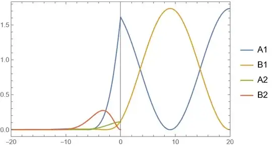
Block[{x1 = -20, x2 = 20, En = Re@Eng[[1, 2]]}, 
 Show[Plot[{Abs[A[x]^2], (Abs@B[x])^2}, {x, 0, x2}, Frame -> True, 
       PlotRange -> {{x1, x2}, All}], 
  Plot[{(Abs@A1[x])^2, (Abs@B1[x])^2, (Abs@A2[x])^2, (Abs@
      B2[x])^2}, {x, x1, 0},  
   Frame -> True, PlotRange -> All, 
   PlotLegends -> {"A1", "B1", "A2", "B2"}]]]    

Answer 1

"Different equations for different region" is not directly supported by NDSolve, NDEigensystem, etc. (at least for now), but in many cases, the different PDEs can be combined to one PDE with piecewise coefficients, and your problem luckily belongs to such cases. The following is a solution that at least produces a solution:

{a = 400, hv = 0.65875 10^3, W = 23.86, k = 0., inf = 2 W, bR = 10 W};
<< NDSolve`FEM`;
meshline = 
  ToElementMesh[ImplicitRegion[-inf <= x <= bR, x], {{-inf, bR}}, 
   IncludePoints -> {{0}}, MaxCellMeasure -> 1];
eps = 10^-3;
{val, vec} = NDEigensystem[Flatten@{
     hv (-B1'[x] - k B1[x]) + If[x < 0, 50, 0] A1[x] + eps A1''[x],
     hv (A1'[x] - k A1[x]) + If[x < 0, 50, 0] B1[x] + If[x < 0, a, 0] A2[x] + 
      eps B1''[x],
     hv (B2'[x] + k B2[x]) - 50 A2[x] + a B1[x] + eps A2''[x],
     hv (-A2'[x] + k A2[x]) - 50 B2[x] + eps B2''[x],
     DirichletCondition[B2[x] == 0, x == 0],
     DirichletCondition[B1[x] == 0, x == bR],
     DirichletCondition[#, x == -inf] & /@ {A1[x] == 0, B1[x] == 0, A2[x] == 0, 
       B2[x] == 0}}, {A1, B1, A2, B2}, {x} ∈ meshline, 6];

Eigensystem::chnpdef: Warning: there is a possibility that the second matrix SparseArray[...] in the first argument is not positive definite, which is necessary for the Arnoldi method to give accurate results.

Further check shows the b.c. at x == bR isn't satisfied. Other b.c.s are satisfied well, though:

index = 3;
{vec[[index, 2]][bR], vec[[index, 4]][0], vec[[index]][-inf] // Through}
(* {163.436 - 136.252 I, 
    5.5511210^-17 + 1.9428910^-16 I, 
   {0. + 0. I, 0. + 0. I, 0. + 0. I, 0. + 0. I}} *) 

I'm not familiar with the corresponding physics background and haven't looked into the linked paper so cannot tell what's wrong, but I'd suggest double-checking if the system itself is correct as the next step.

Remark

1. The IncludePoints -> {{0}} is necessary for the boundary condition at x == 0.

2. Since the equations for A1 and A, B1 and B are combined, the junction conditions A1[0]==A[0], B1[0]==B[0] are automatically satisfied and don't need to be set explicitly.

3. The eps is to suppress the NDEigensystem::femcscd warning, taking it away doesn't influence the solution much actually.

---

FDM based solution

FEM is having difficulty with the problem, so let me add a finite difference method (FDM) based solution. Here I'm solving the system in update 3 so we can compare with the deduced analytic solution. As usual, I'll use pdetoae for generation of difference equations:

{xL, xR} = {-20, 20};
vars = {A1, B1, A2, B2};
unitStepExpand = Simplify`PWToUnitStep@PiecewiseExpand@# &;
oper = {-B1'[x] + u A1[x],
  A1'[x] + u B1[x] + unitStepExpand@If[x < 0, 1, 0] A2[x],
  B2'[x] - u A2[x] + B1[x],
  -A2'[x] - u B2[x]}
intervals = 500; points = intervals + 1; mid = intervals/2 + 1; 
grid = Subdivide[xL, xR, intervals]; difforder = 8;
(* Definition of pdetoae isn't included in this post,
   please find it in the link above. *)
ptoafunc = pdetoae[vars[x], grid, difforder];
disvars = Flatten@Outer[#[#2] &, vars, grid];
marray = CoefficientArrays[ptoafunc@oper // Flatten, disvars] // Last;
(* Impose the Dirichlet b.c.: *)

pos = {1, points + 1, 2 points + 1, 3 points + 1, 2 points, 3 points + mid};

(marray[[#, All]] = 0) & /@ pos;
{val, veclst} = 
  Block[{u = 1/8}, Eigensystem[N[marray], 6, Method -> {"Arnoldi", "Shift" -> -0.1}]];
val
(* {-0.18626, -0.168633, -0.136571, -0.122453 + 0.000729685 I, -0.122453 - 
     0.000729685 I, -0.0183314} *)
vec = (ListInterpolation[#, grid] & /@ Partition[#, points]) & /@ veclst;
Block[{A1, B1, A2, B2}, {A1, B1, A2, B2} = #; 
   Show[Plot[{A1[x], B1[x]}^2 // Abs // Evaluate, {x, 0, xR}, Frame -> True, 
     PlotRange -> {{xL, xR}, All}], 
    Plot[Through[{A1, B1, A2, B2}[x]]^2 // Abs // Evaluate, {x, xL, 0}, 
     PlotRange -> All, PlotLegends -> {"A1", "B1", "A2", "B2"}]]] & /@ vec

As we can see, this method is far beyond perfect: the graphics of corresponding eigenvectors indicate the first 5 eigenvalues are fake. Nevertheless, the last eigenvalue is clearly the one found analytically by OP.

Remark

1. The "Shift" sub-option is critical for this solution.

2. difforder = 2 can be used, but then we need to set an even closer "Shift" e.g. "Shift" -> -0.01.

3. If we take the issue discussed in the tutorial Ordering of Dependent Variable Names into account, the FEM solution will satisfy all the b.c.s, but still, the eigenvectors are rather inaccurate (incorrect?). The following is my failed trial:

   meshline = 
     NDSolve`FEM`ToElementMesh[ImplicitRegion[xL <= x <= xR, x], {{xL, xR}}, 
      IncludePoints -> {{0}}, MaxCellMeasure -> .02];
   bcL = DirichletCondition[#[x] == 0, x == xL] & /@ vars;
   Block[{u = 1/8},
     {val, vec} = 
      NDEigensystem[
       oper + bcL + {0, DirichletCondition[B1[x] == 0, x == xR], 0, 
                     DirichletCondition[B2[x] == 0, x == 0]} // Flatten,
       vars, {x} ∈ meshline, 6, Method -> {"Arnoldi", "Shift" -> -0.018}]];
   val
   Map[vec |-> {vec[[2]][xR], vec[[4]][0], vec[xL] // Through}]@vec
   (* Very close to 0. *)
   

---

Addendum: Mathematica Aided Deduction for the Symbolic Solution

The following is a deduction for the analytic solution shown by OP with the help of Mathematica. We first find the general solutions of the system:

eq = {-B1'[x] + u A1[x] == En A1[x],
   A1'[x] + u B1[x] + A2[x] == En B1[x],
   B2'[x] - u A2[x] + B1[x] == En A2[x],
   -A2'[x] - u B2[x] == En B2[x],
   -B'[x] + u A[x] == En A[x],
   A'[x] + u B[x] == En B[x]};
vars = {A1, B1, A2, B2, A, B};
sol = DSolve[eq, vars[x] // Through, x][[1]] // Expand // Collect[#, Exp[_]] &

By observing sol, we see A1, B1, A2, B2 are summation of _ Exp[Sqrt[_]] and _ Exp[-Sqrt[_]]. Since A1, B1, A2, B2 vanish at $-\infty$, and:

Reduce[ForAll[{a, b}, {a, b} ∈ Reals, Re@Sqrt[a + b I] >= 0]]
(* True *)

We know the coefficients of A1, B1, A2, B2 in form Exp[-_] should be zero:

term = Cases[sol[[;; 4]], a_ Exp[-_] :> a, Infinity] // Simplify // Union;
const = Cases[sol[[;; 4]], C[_], Infinity] // Union
(* {C[1], C[2], C[3], C[4]} *)
rulec1 = Solve[term == 0, const] // Flatten;
constrest = 
 Complement[Cases[sol, C[_], Infinity] // Union, rulec1[[All, 1]]]
(* {C[1], C[2], C[5], C[6]} *)

Using the b.c. at $-\infty$, we manage to eliminate C[3] and C[4]. We continue to determine the rest 4 constants with the other 4 b.c.s:

{xL, xR} = {-20, 20};
bcsys = {A[x] == A1[x] /. sol /. x -> 0,
    B[x] == B1[x] /. sol /. x -> 0,
    B[x] == 0 /. sol /. x -> xR,
    B2[x] == 0 /. sol /. x -> 0} /. rulec1;

Reduce[bcsys, constrest] should work in principle, but it's too slow, so we still follow OP's method to find non-trivial solution:

det[u_, En_] = CoefficientArrays[bcsys, constrest] // Last // Det;

By observing

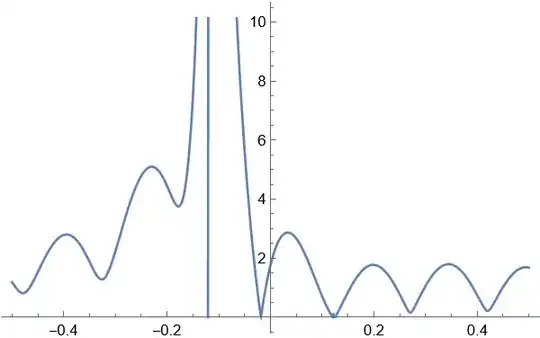
Plot[det[1/8, En] // Abs // Evaluate, {En, -1/2, 1/2}]

Or directly use RootSearch:

ruleEn = RootSearch[det[1/8, En] == 0, {En, -1/2, 1/2}]
(* {{En -> -0.120949}, {En -> -0.0184422}, {En -> 0.12101}} *)

We see there seem to be 3 possible En. Let's check the corresponding eigenvalues:

rulec2 = FindInstance[bcsys /. # /. u -> 1/8, constrest, 2][[1]] & /@ ruleEn
solfinal = 
  MapThread[sol[[All, -1]] /. rulec1 /. # /. u -> 1/8 /. #2 &, {rulec2, ruleEn}];
MapThread[Plot[#^2 // Abs // Evaluate, {x, xL, 0}, PlotRange -> All]~Show~
          Plot[#2^2 // Abs // Evaluate, {x, 0, xR}, PlotRange -> All] &, 
          {solfinal[Transpose][[;; 4]][Transpose], 
           solfinal[Transpose][[5 ;;]][Transpose]}]

Only eigenvectors of En -> -0.0184422 satisfy the b.c.s at $-\infty$, so it seems to be the only valid eigenvalue.

This deduction is fully applicable for $k\neq 0$ case. If you just need to solve the problem, perhaps it's better to forget about numeric approach and stay with symbolic approach.

Answer 2

Update: I have updated my package to be able to work on this system, fixing the bugs I noted in my previous answer.

I have a package for solving eigenvalue boundary value problems using the method of compound matrices, that is suitable here. I have answered a number of other questions on this site using it(e.g. interface eigenvalue BVP question) although I haven't been actively working in this area for several years so development has stopped. The package github holds the package, including a Mathematica notebook with a number of worked examples. This search contains all the answers I have made on this site.

First, we install the most recent v0.9.2 version of the package:

Needs["PacletManager`"]
PacletInstall["https://github.com/SPPearce/CompoundMatrixMethod/raw/master/\
CompoundMatrixMethod-0.92.paclet"]

We need to transform the equations into a matrix system of first order equations, including the boundary conditions, i.e. as:

\begin{align} \mathbf{A}_y(\lambda, x) \cdot \mathbf{y} &= \frac{d \mathbf{y}}{dx}, \quad x_1 \leq x \leq x_2 \\ \mathbf{A}_z(\lambda, x) \cdot \mathbf{z} &= \frac{d \mathbf{z}}{dx}, \quad x_2 \leq x \leq x_3 \\ \\ \mathbf{B} \cdot \mathbf{y}(x_1) &= \mathbf{0}, \\ \mathbf{F} \cdot \mathbf{y}(x_2) +\mathbf{G} \cdot\mathbf{z}(x_2) &= \mathbf{0}, \\ \mathbf{C} \cdot \mathbf{z}(x_3) &= \mathbf{0}. \\ \end{align}

for some matrices $\mathbf{A}_y, \mathbf{A}_z, \mathbf{B}, \mathbf{C}, \mathbf{F}, \mathbf{G}$, which may all involve the eigenvalue $\lambda$ (and $\mathbf{A}_y$ and $\mathbf{A}_z$ may be functions of $x$).

Fortunately, the package has a function to do that, ToMatrixSystem, so we can do that automatically.

So we can setup your (reduced) equations and apply them:

Needs["CompoundMatrixMethod`"]
eqnLeft = {-B1'[x] + u A1[x] == λ  A1[x],
   A1'[x] + u B1[x] + A2[x] == λ  B1[x],
   B2'[x] - u A2[x] + B1[x] == λ  A2[x],
   -A2'[x] - u B2[x] == λ  B2[x]};
eqnRight = {(-B'[x]) + u A[x] == λ A[x], 
  A'[x] + u B[x] == λ B[x]};
BCsRight = {B[W] == 0};
BCsInterface = {A1[0] == A[0], B1[0] == B[0], B2[0] == 0};

We will discuss the left-hand BCs later.

Now we will basically integrate from both the left-hand side, $x=x_a$, and the right-hand side, $x=x_c$, and meet in the middle with the matching condition. However, this is easier to do numerically if we transform to a higher-order manifold, by introducing compound matrices. I'm not going to go into the details here, as the package takes care of that, but there is a helpful explanation by my former PhD supervisor.

We end up with what is known as the Evans function (denoted $E(\lambda)$, or miss-distance function, that basically describes how far off the matching at the middle we are.

The left-hand BCs here is that they decay to zero. Now we could choose a pair of the functions to set to zero here, or we can formally require decay conditions. As $x \to -\infty$, the system will behave as a constant $\mathbf{y}' = \mathbf{A}_{y\inf}(\lambda)$, and so has an exponential solution, $\mathbf{y} = \sum_i \exp(- \xi_i x) \mathbf{y}_i^{-\inf}$, where $\xi_i$ and $\mathbf{y}_i^{-\inf}$ are the matrix eigenvalues and eigenvectors respectively. For $y$ to decay therefore, we require that only the eigenvalues with negative real parts of this matrix remain, else we'll have exponentially growing terms. So the boundary condition here is the $\mathbf{B}$ is the concatenation of these two eigenvectors corresponding to eigenvalues with negative real parts.

My package will assume missing boundary conditions are of this form, so we just provide:

sys = ToMatrixSystem[{eqnLeft, eqnRight}, {BCsRight, 
  BCsInterface}, {{A1, B1, A2, B2}, {A, B}}, {x, -L, 0, W}, λ]

Which spits out this, containing the matrices required. Note the {}, which is the missing boundary conditions to be filled in later.

{{{{0, \[FormalLambda] - u, -1, 0}, {-\[FormalLambda] + u, 0, 0, 
    0}, {0, 0, 0, -\[FormalLambda] - u}, {0, -1, \[FormalLambda] + u, 
    0}}, {{0, \[FormalLambda] - u}, {-\[FormalLambda] + u, 
    0}}}, {}, {{0, 1}}, {{{1, 0, 0, 0}, {0, 1, 0, 0}, {0, 0, 0, 1}}, {{-1, 0}, {0, -1}, {0, 0}}}, {x, -L, 0, W}}

Here \[FormalLambda] is the eigenvalue in this system.

Now we can put this into the second function in the package, Evans, to calculate $E(\lambda)$ for a given possible eigenvalue $\lambda$.

So we can evaluate the system with $u = 1/8$, right hand boundary $x_3 = W = 20$ and apply the left-hand boundary condition at $x_1 = L = -20$, and give a possible eigenvalue of $\lambda = 0$:

 Evans[0, sys /. {W -> 20, L -> 20, u -> 1/8}]
 (* -3.97135 + 2.13421*10^-17 I *)

This value is not zero, so $\lambda = 0$ is not an eigenvalue. We can then use FindRoot,

FindRoot[Evans[λ, sys /. {W -> 20, L -> 20, u -> 1/8}], {λ, 0}]
(* {λ -> -0.0184414 - 5.66513*10^-17 I} *)

to recover the analytically found eigenvalue.

We can also plot this function, to see how it behaves, showing one eigenvalue here.

Plot[Evans[λ, sys /. {W -> 20, L -> 20, u -> 1/8}], {λ, -0.1, 0.1}]

Note that there will be (possibly large) regions of parameter space where we can't apply this function because the matrix eigenvalues are purely imaginary. This is not caught gracefully and will just give you an error I'm afraid. The first part of the system is the matrix $\mathbf{A}_y$:

sys[[1, 1]] // MatrixForm

and you can look at what points the eigenvalues of this matrix are not purely imaginary.

This method should also work for the $k \neq 0 $ case, but I haven't tried that yet.