Understanding the calculation of the periodic function $f(x)=x-x^3, \quad -1

Question

It is given the following periodic function $$f(x)=x-x^3, \quad -1<x<1$$ This is an odd function, so the coefficients $a_n,a_0$ of the Fourier Series are zero.

Usually, I face function with two branches so I tried to code it on Mathematica as follows:

f[x_] := Which[-1 < x <= 0, x - x^3, 0 < x < 1, x - x^3]
Plot[f[x], {x, -1, 1}]

Edited

a[n_] := (2/L)*Integrate[f[x]*Cos[2 n*Pi*x/L], {x, -L/2, L/2}]
a[0] := (1/L)*Integrate[f[x], {x, -L/2, L/2}]
b[n_] := (2/L)*Integrate[f[x]*Sin[2 n*Pi*x/L], {x, -L/2, L/2}]
F[x_, Nmax_] := 
 a[0] + Sum[a[n]*Cos[2 n*Pi*x/L] + b[n]*Sin[2 n*Pi*x/L], {n, 1, N}]
p[Nmax_, a_] := 
 Plot[Evaluate[F[x, Nmax]], {x, -a, a}, PlotRange -> All, 
  PlotPoints -> 200]
L = 2;
f[x_] := If[x > 0, x - x^3, x - x^3];
a[n]
a[0]
b[n]
Simplify[b[n], n \[Element] Integers]
Integrate[f[x]^2, {x, -L, L}]
(a[0]^2)/2 + Sum[(a[n]^2 + b[n]^2), {n, 1, Infinity}] <= 
 Integrate[f[x]^2, {x, -L, L}]

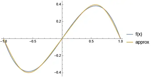
Is my consideration correct? I can realize that the two plots are the same and for this reason seems weird.

f[x_] := Which[-1 < x <= 0, x - x^3, 0 < x < 1, x - x^3] is equivalent to: f[x_]:= x - x^3 — Daniel Huber, Jan 19 '23 at 10:29
You should not use N as variable. Also, please clarify what is your question more clearly. Are you asking if your Fourier series manual calculations correct or not? — Nasser, Jan 19 '23 at 10:30
@Nasser I used it as my professor showed us. I did not know that is wrong. Yes, I am asking if the calculation is correct. Here, I can realize that we have a continuous function. So there is no Gibbs Phenomenon. — Athanasios Paraskevopoulos, Jan 19 '23 at 10:38
For reference: Fourier series in Mathematica video tutorial. — Syed, Jan 19 '23 at 10:48
Expanding on what @Nasser told you. Some capital letters in Mathematica are built-in symbols. If you don't remember which ones, don't use any. For example you could have written NN instead of N as your variable. You can test. Try ?? N and see what you get. To avoid this test here's a simple mnemonic. Don't use ONE DICK; shameless advertising see here and the linked one — bmf, Jan 19 '23 at 10:52
Can the downvoter explain the reasoning behind the vote? It would be more beneficial to the author of the O.P. Also, I don't see any reason for a downvote. It's a clear question and some effort was made. Code was provided. The post is nicely formatted. And I can go on... — bmf, Jan 19 '23 at 11:39
@bmf Understood I have to be more careful with the variables. I will fix it. Is there any answer for my question why the two plots are identical? — Athanasios Paraskevopoulos, Jan 19 '23 at 11:52
@AthanasiosParaskevopoulos sorry. I did not have the time to check. — bmf, Jan 19 '23 at 11:56
@bmf I have changed the variables as you said to me. If you have the time to check it I would deeply appreciate it. — Athanasios Paraskevopoulos, Jan 19 '23 at 11:59
@AthanasiosParaskevopoulos I was about to explain the same thing that Nasser explained to you. They are not identical for low values, but they are really close — bmf, Jan 19 '23 at 12:21

score 2 · Accepted Answer · answered Jan 19 '23 at 12:06

is this the reason that the plots are identical?

They are not identical. But the approximation is very good. Even for 2 terms, you get very good approximation. You can see this as below

L = 2; (*period*)
f[x_] := x - x^3;
a[n_, x_] = (2/L)*Integrate[f[x]*Cos[2 n*Pi*x/L], {x, -L/2, L/2}]
a[n_ /; n == 0, x_] = (1/L)*Integrate[f[x], {x, -L/2, L/2}]
b[n_, x_] = (2/L)*Integrate[f[x]*Sin[2 n*Pi*x/L], {x, -L/2, L/2}]

Mathematica graphics

Notice also since odd function, only $b_n$ survives.

fFourierApprox[x_, nTerms_] := 
  a[0, x] + Sum[a[n, x]*Cos[2 n*Pi*x/L] + b[n, x]*Sin[2 n*Pi*x/L], {n, 1,  nTerms}];

Let compare $f(x)$ with its Fourier series, using one term only

Plot[{f[x], fFourierApprox[x, 1]}, {x, -L/2, L/2}, 
 PlotLegends -> {"f(x)", "approx"}, PlotRange -> All]

Mathematica graphics

Using 2 terms now

Plot[{f[x], fFourierApprox[x, 2]}, {x, -L/2, L/2}, 
 PlotLegends -> {"f(x)", "approx"}, PlotRange -> All]

Mathematica graphics

With 3 terms you can hardly see the difference

Plot[{f[x],fFourierApprox[x,3]},{x,-L/2,L/2},PlotLegends->{"f(x)","approx"},PlotRange->All]

Mathematica graphics

You original function is continuous, so as typical in Fourier series, few terms are needed to give very accurate approximation. (There are more Fourier series animations showing this point all done using Mathematica I saw at this page)

ps. If you extend the range to the full -L..L, this is the result using only one term in F.S.

Plot[{f[x], fFourierApprox[x, 1]}, {x, -L, L}, 
 PlotLegends -> {"f(x)", "approx"}, PlotRange -> All]

Mathematica graphics

Oh thank you. I was so confused. I have to compare them – Athanasios Paraskevopoulos Jan 19 '23 at 12:27 — Athanasios Paraskevopoulos, Jan 19 '23 at 12:27

Understanding the calculation of the periodic function $f(x)=x-x^3, \quad -1

1 Answers1