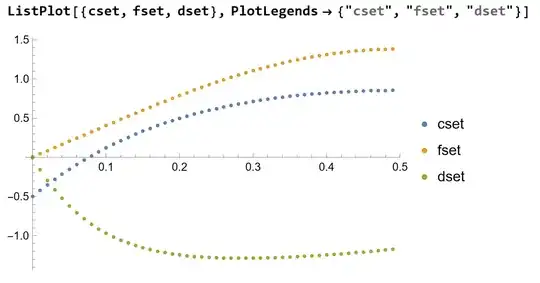
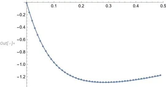
Step size issue with ParametricNDSolveValue to fit data to a set of non linear differential equations

Question

I am fitting dataset dset to a set of non-linear differential equations to find the fitting parameters dP (pressure differential) and LK (thermodynamic tension)

dset = {{0.0005`, -0.010556322978021847`}, {0.010500000000000006`, \
-0.16182647440121997`}, {0.020500000000000015`, \
-0.29695349218330797`}, {0.030500000000000024`, \
-0.4182634329865751`}, {0.04050000000000003`, -0.5269223967724705`}, \
{0.05050000000000004`, -0.6240338483581807`}, {0.06050000000000005`, \
-0.7106407676192987`}, {0.07050000000000005`, -0.7877204571404507`}, \
{0.08050000000000006`, -0.856181218817242`}, {0.09050000000000007`, \
-0.9168613181414874`}, {0.10050000000000008`, -0.9705298179210835`}, \
{0.11050000000000008`, -1.0178887965803456`}, {0.1205000000000001`, \
-1.059576525235709`}, {0.1305000000000001`, -1.096171257192166`}, \
{0.1405000000000001`, -1.1281953593331848`}, {0.1505000000000001`, \
-1.1561195807387954`}, {0.16050000000000011`, -1.1803673085219024`}, \
{0.17050000000000012`, -1.2013187048750018`}, {0.18050000000000013`, \
-1.219314653893368`}, {0.19050000000000014`, -1.2346604733142499`}, \
{0.20050000000000015`, -1.247629366294407`}, {0.21050000000000016`, \
-1.2584656030266932`}, {0.22050000000000017`, -1.2673874324894605`}, \
{0.23050000000000018`, -1.2745897318716903`}, {0.24050000000000019`, \
-1.2802464059943979`}, {0.25050000000000017`, -1.284512551975971`}, \
{0.2605000000000002`, -1.2875264059562497`}, {0.2705000000000002`, \
-1.2894110892831467`}, {0.2805000000000002`, -1.2902761714693076`}, \
{0.2905000000000002`, -1.2902190666663456`}, {0.3005000000000002`, \
-1.289326279545788`}, {0.3105000000000002`, -1.2876745154405251`}, \
{0.32050000000000023`, -1.2853316684758496`}, {0.33050000000000024`, \
-1.2823577002670472`}, {0.34050000000000025`, -1.2788054206235198`}, \
{0.35050000000000026`, -1.2747211806057743`}, {0.36050000000000026`, \
-1.2701454872488802`}, {0.3705000000000003`, -1.2651135483041822`}, \
{0.3805000000000003`, -1.259655754464611`}, {0.3905000000000003`, \
-1.2537981057286822`}, {0.4005000000000003`, -1.2475625878223087`}, \
{0.4105000000000003`, -1.2409675039324466`}, {0.4205000000000003`, \
-1.2340277664078854`}, {0.4305000000000003`, -1.2267551525451035`}, \
{0.44050000000000034`, -1.2191585280958825`}, {0.45050000000000034`, \
-1.2112440417030041`}, {0.46050000000000035`, -1.2030152930855527`}, \
{0.47050000000000036`, -1.1944734774498176`}, {0.48050000000000037`, \
-1.1856175082766092`}, {0.4905000000000004`, -1.1764441200214577`}};
fset = {{0.0005, 0.0029994884862318545}, {0.010500000000000006, 0.04290422551646877}, {0.020500000000000015, 0.08271521578894832}, {0.030500000000000024, 0.1225075890771862}, {0.04050000000000003, 0.16232844620349135}, {0.05050000000000004, 0.2022016182928511}, {0.06050000000000005, 0.24213173178259795}, {0.07050000000000005, 0.2821076803700469}, {0.08050000000000006, 0.32210558852161697}, {0.09050000000000007, 0.36209133779687963}, {0.10050000000000008, 0.4020227165941489}, {0.11050000000000008, 0.44185124530069814}, {0.1205000000000001, 0.4815237217048463}, {0.1305000000000001, 0.5209835255288894}, {0.1405000000000001, 0.5601717158155678}, {0.1505000000000001, 0.599027950470219}, {0.16050000000000011, 0.6374912534028201}, {0.17050000000000012, 0.6755006513403476}, {0.18050000000000013, 0.7129956994240441}, {0.19050000000000014, 0.7499169121163021}, {0.20050000000000015, 0.7862061136751125}, {0.21050000000000016, 0.8218067204737102}, {0.22050000000000017, 0.8566639657168472}, {0.23050000000000018, 0.8907250756040312}, {0.24050000000000019, 0.9239394046879505}, {0.25050000000000017, 0.9562585370494301}, {0.2605000000000002, 0.9876363589372191}, {0.2705000000000002, 1.0180291076824612}, {0.2805000000000002, 1.0473954009765578}, {0.2905000000000002, 1.075696249981966}, {0.3005000000000002, 1.1028950592146718}, {0.3105000000000002, 1.1289576156826286}, {0.32050000000000023, 1.1538520693758882}, {0.33050000000000024, 1.1775489068722165}, {0.34050000000000025, 1.200020919538734}, {0.35050000000000026, 1.2212431675685949}, {0.36050000000000026, 1.241192940885903}, {0.3705000000000003, 1.2598497177767924}, {0.3805000000000003, 1.277195121955397}, {0.3905000000000003, 1.2932128786464807}, {0.4005000000000003, 1.3078887701584572}, {0.4105000000000003, 1.3212105913286585}, {0.4205000000000003, 1.3331681051444677}, {0.4305000000000003, 1.343752998777381}, {0.44050000000000034, 1.3529588402103094}, {0.45050000000000034, 1.3607810355900682}, {0.46050000000000035, 1.3672167873955854}, {0.47050000000000036, 1.372265053476814}, {0.48050000000000037, 1.375926506987712}, {0.4905000000000004, 1.3782034971952344}};
cset = {{0.0005, -0.5042310407443639}, {0.010500000000000006, \ -0.427674601050752}, {0.020500000000000015, -0.3544091437700765}, 

{0.030500000000000024, -0.28474223380967734}, 

{0.04050000000000003, -0.21845219304523977}, {0.05050000000000004, \ -0.1553452433932613}, {0.06050000000000005, -0.09525380897089007}, 

{0.07050000000000005, -0.038030681942581725}, {0.08050000000000006, 0.016455923730000113}, {0.09050000000000007, 0.0683261356767569}, {0.10050000000000008, 0.11769117737156293}, {0.11050000000000008, 0.164655332408679}, {0.1205000000000001, 0.2093173133085545}, {0.1305000000000001, 0.25177119317041247}, {0.1405000000000001, 0.29210702401667615}, {0.1505000000000001, 0.33041123620685403}, {0.16050000000000011, 0.36676688931358775}, {0.17050000000000012, 0.4012538259126424}, {0.18050000000000013, 0.43394876511503755}, {0.19050000000000014, 0.4649253615923762}, {0.20050000000000015, 0.49425424760155606}, {0.21050000000000016, 0.5220030694835737}, {0.22050000000000017, 0.5482365257784656}, {0.23050000000000018, 0.5730164110488714}, {0.24050000000000019, 0.5964016674098069}, {0.25050000000000017, 0.6184484443671279}, {0.2605000000000002, 0.6392101666770944}, {0.2705000000000002, 0.6587376094076599}, {0.2805000000000002, 0.677078979099448}, {0.2905000000000002, 0.6942799998106967}, {0.3005000000000002, 0.7103840028276676}, {0.3105000000000002, 0.7254320188886919}, {0.32050000000000023, 0.7394628718770215}, {0.33050000000000024, 0.7525132730649463}, {0.34050000000000025, 0.764617915125826}, {0.35050000000000026, 0.7758095652630415}, {0.36050000000000026, 0.7861191569301358}, {0.3705000000000003, 0.7955758797315625}, {0.3805000000000003, 0.8042072671971728}, {0.3905000000000003, 0.8120392822155327}, {0.4005000000000003, 0.8190963999917696}, {0.4105000000000003, 0.8254016884657382}, {0.4205000000000003, 0.8309768861869055}, {0.4305000000000003, 0.8358424776946949}, {0.44050000000000034, 0.8400177664982754}, {0.45050000000000034, 0.8435209457891544}, {0.46050000000000035, 0.8463691670545794}, {0.47050000000000036, 0.8485786067907134}, {0.48050000000000037, 0.8501645315425272}, {0.4905000000000004, 0.8511413615178258}};

below are the equations and the model for fitting the data

c0 = -4.0;
eqn1 = c'[s] == (-2 d[s] Sqrt[1 - f[s] c[s]^2])/f[s];
eqn2 = f'[s] == 4 Sqrt[1 - f[s] c[s]^2];
eqn3 = d'[s] == -(2 c[s]^2 (d[s] - c0) + c[s] (c0^2 - d[s]^2) + LK c[s] + 
      dP + 4 d[s] (1 - f[s] c[s]^2)/f[s])/Sqrt[1 - f[s] c[s]^2];
system = {eqn1, eqn2, eqn3, f[0.0005] == 0.0029994884862318545, d[0.0005] == -0.010556322978021847, c[0.0005] == -0.5042310407443639`};
model = ParametricNDSolveValue[system, d, {s, 0.0005, 0.5}, {dP, LK}, MaxSteps -> Infinity];

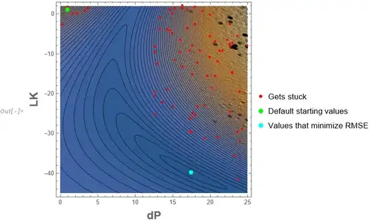
I get an error in execution when I try to use the entire dset for fitting. And although I get the correct fitting parameter values for dP and LK, this happens when I use a subset i.e. dset[[;;ind]] where ind is less than 38; in this case when the evaluation occurs, I get a complaint that the step size effectively goes to 0 at a particular value of s.

fit = NonlinearModelFit[dset[[1 ;; 37]], model[dP, LK][s], {dP, LK}, s, Method -> "Gradient"];
(*ParametricNDSolveValue::ndsz: At s == 0.37654293376950654`, step size is effectively zero; singularity or stiff system suspected.*)
fit["BestFitParameters"]
{dP -> 17.48, LK -> -39.9968} (*these values are correct as dset, fset and cset were generated using these fitting parameters*)

My question is how to avoid the step size from reaching zero and possibly use the entire dataset dset for fitting?

How long does it take to run the fit =NonlinearModelFit[dset.....? — bmf, Feb 18 '23 at 05:28
@bmf with full dset NonlinearModelFit does not execute. Try dset[[;;36] — Ali Hashmi, Feb 18 '23 at 07:54
@AliHashmi It is not clear why do you use dset only, while model depends on c and f as well? — Alex Trounev, Feb 18 '23 at 08:08
@AlexTrounev I tried using all the three including cset and fset but could not get the code to work. Do you have an idea how to incorporate them as well and make the function work. Thanks ! — Ali Hashmi, Feb 18 '23 at 08:11
@AlexTrounev i even tried this approach of putting cset, fset and dset together but it seems that the solver get stuck. https://mathematica.stackexchange.com/questions/28461/how-to-fit-3-data-sets-to-a-model-of-4-differential-equations — Ali Hashmi, Feb 18 '23 at 09:11

JimB · Answer 1 · 2023-02-20T22:11:11.533

Good starting values are your best friends. If you start with {{dP, 17}, {LK, -41}} and use all of the data, then NonlinearModelFit executes quickly with only one minor warning:

A plot of the fit is

Show[ListPlot[dset], Plot[fit[s], {s, Min[dset[[All, 1]]], Max[dset[[All, 1]]]}, PlotRange -> All]]

The estimated root mean square error is

Sqrt[fit["EstimatedVariance"]]
(* 5.89791*10^-8 *)

Is that close enough to zero for your objective?

The parameter estimators are highly correlated and that many times spells trouble for getting convergence and/or avoiding warning messages.

fit["CorrelationMatrix"] // MatrixForm

Further investigation

It might be closer to the truth that "avoiding some starting values" rather than "choosing starting values closer to the optimal values" is the determining factor. Typically, "closer to the optimal values" is needed to avoid getting lost in a bumpy/treacherous log likelihood surface. But that doesn't seem to be the case here.

The problem seems to be that there are certain pairs of $dP$ and $LK$ that never return a value for model[dP, LK][s] and therefore stop NonlinearModelFit from completing.

Rather than the log likelihood surface, I'll construct the equivalent root mean square error for various pairs of dP and LK. To avoid getting stuck with annoying pairs of dP and LK, the TimeConstrained function will be used to skip the troublemakers after some fixed amount of time.

rmse[dP_?NumericQ, LK_?NumericQ] := 
 Sqrt[Sum[(dset[[i, 2]] - model[dP, LK][dset[[i, 1]]])^2, 
 {i, Length[dset]}]/(Length[dset] - 2)]

Generate values to use in ListContourPlot:

t = ConstantArray[{-1, -1, -1}, 15000];
k = 0;
Do[
  Do[
   k = k + 1;
   t[[k]] = {dP, LK, TimeConstrained[rmse[dP, LK], 0.1, -2]},
   {dP, 0, 25, 1/3}],
  {LK, -45, 2, 1/3}];
tGood = Select[t, #[[3]] > 0 &];
tBad = Select[t, #[[3]] == -2 &];

Show results:

Show[ListContourPlot[tGood, Contours -> 100, PlotRange -> All,
  Frame -> True, FrameLabel -> (Style[#, Bold, 18] &) /@ {"dP", "LK"}],
 ListPlot[{tBad[[All, {1, 2}]], {{1, 1}}, {{17.5, -39.9}}}, 
  PlotStyle -> {Red, {PointSize[0.02], Green}, {PointSize[0.02],  Cyan}},
  PlotLegends -> {"Gets stuck", "Default starting values", "Values that minimize RMSE"}]]

An example of a set of parameter values that gets stuck is

model[21, -31][30]

I don't know why.

{{dP, 5}, {LK, -1}} works well, too, as starting values. I suppose telling NonlinearModelFit that LK could be negative is the most influential reason for convergence given the high negative correlation between the two parameter estimators. — JimB, Feb 19 '23 at 19:18
the staring range like {{dP,5}, {LK,-1}} can work as well for starting values. The only issue is that when fitting sometimes one may not even know a good defining range for the parameters. Can you let me know how can you define LK < 0 as a constraint in NonlinearModelFit? Perhaps this suggestion of yours can be incorporated in the answer that I have posted below — Ali Hashmi, Feb 20 '23 at 10:20
You can change model[dP, LK][s] to {model[dP, LK][s], LK < 0} but you'll also need to give an explicit negative starting value as the default starting values are all 1. The documentation for NonlinearModelFit has more details. — JimB, Feb 20 '23 at 18:20
i will go through your answer in detail especially the choice of starting values. thanks ! — Ali Hashmi, Feb 24 '23 at 12:09

Ali Hashmi · Answer 2 · 2023-02-18T21:54:27.370

Not a complete answer that I was looking for but based on @AlexTrounev 's comment, I added dset and cset for fitting the model. Addition of fset was causing trouble - I do not know the reason why - so I omitted it from the fitting procedure. I tried with various methods and the code below seems to work fine. Moreover, I added Method -> {"StiffnessSwitching", Method -> {"ExplicitRungeKutta", Automatic}} to ParametricNDSolve.

Why I can only take partial subset of the entire dataset for the fitting procedure is still a mystery to me (here I take values for which abscissa s < 0.25. All procedures give the correct fits for this cutoff. Except for InteriorPoint and Newton all other methods give the correct fitting parameters until s < 0.30)

c0 = -4.0;
eqn1 = c'[s] == (-2 d[s] Sqrt[1 - f[s] c[s]^2])/f[s];
eqn2 = f'[s] == 4 Sqrt[1 - f[s] c[s]^2];
eqn3 = d'[
    s] == -(2 c[s]^2 (d[s] - c0) + c[s] (c0^2 - d[s]^2) + LK c[s] + 
      dP + 4 d[s] (1 - f[s] c[s]^2)/f[s])/Sqrt[1 - f[s] c[s]^2];
system = {eqn1, eqn2, eqn3, f[fset[[1, 1]]] == fset[[1, 2]], 
   d[dset[[1, 1]]] == dset[[1, 2]], c[cset[[1, 1]]] == cset[[1, 2]]};
sol = ParametricNDSolveValue[
  system, {c, d}, {s, 0.0005, 0.5}, {dP, LK}, MaxSteps -> Infinity, 
  Method -> {"StiffnessSwitching", 
    Method -> {"ExplicitRungeKutta", Automatic}}]
abscissae = dset[[All, 1]];
data = {cset[[All, 2]], dset[[All, 2]]};
transformedData = {ConstantArray[Range@Length[data],Length[abscissae]]//Transpose, 
    ConstantArray[abscissae, Length[data]], data}~Flatten~{{2, 3}, {1}};
model[dP_, LK_][i_, s_] := Through[sol[dP, LK][s], List][[i]]/;And@@NumericQ/@{dP, LK, i, s};

here are the methods that I tried in NonlinearModelFit

Monitor[fit = 
   Quiet@NonlinearModelFit[Cases[transformedData, {_, x_ /; x < 0.25, _}], 
     model[dP, LK][i, s], {dP, LK}, {i, s}, Method -> Automatic], {dP,LK}];
fit["BestFitParameters"] (*done*)
{dP -> 17.479913430292985`, LK -> -39.99712108751334`}
Monitor[fit = 
   Quiet@NonlinearModelFit[Cases[transformedData, {, x /; x < 0.25, _}], 
     model[dP, LK][i, s], {dP, LK}, {i, s},Method -> "Gradient"], {dP, LK}];
fit["BestFitParameters"] (done)
{dP -> 17.479912619463647, LK -&gt; -39.99712090614286}
Monitor[fit = 
Quiet@NonlinearModelFit[Cases[transformedData,{, x /; x < 0.25, _}],
 model[dP, LK][i, s], {dP, LK}, {i, s}, Method -> "ConjugateGradient"], {dP,LK}];
fit["BestFitParameters"] (done)
{dP -> 17.4799737562324, LK -&gt; -39.997400761203224}
Monitor[fit = 
   Quiet@NonlinearModelFit[Cases[transformedData, {, x /; x < 0.25, _}], 
     model[dP, LK][i, s], {dP, LK}, {i, s},Method -> "InteriorPoint"], {dP, LK}];
fit["BestFitParameters"] (done)
{dP -> 17.479910658502142, LK -&gt; -39.997119423303715}
Monitor[fit = 
   Quiet@NonlinearModelFit[Cases[transformedData, {, x /; x < 0.25, _}], 
     model[dP, LK][i, s], {dP, LK}, {i, s}, Method -> "Newton"], {dP,LK}];
fit["BestFitParameters"] (done)
{dP -> 17.47991042033268, LK -&gt; -39.99712109812271}
Monitor[fit = 
   Quiet@NonlinearModelFit[Cases[transformedData, {, x /; x < 0.25, _}], 
     model[dP, LK][i, s], {dP, LK}, {i, s},Method -> "LevenbergMarquardt"], {dP,LK}];
fit["BestFitParameters"] (done)
{dP -> 17.479913430292985, LK -&gt; -39.99712108751334}
Monitor[fit = 
   Quiet@NonlinearModelFit[Cases[transformedData, {, x /; x < 0.25, _}], 
     model[dP, LK][i, s], {dP, LK}, {i, s}, Method -> {"NMinimize", Method -> "SimulatedAnnealing"}], {dP,LK}];
fit["BestFitParameters"] (done)
{dP -> 17.479912088798113, LK -&gt; -39.99711877609685}
```

This is very good attempt (+1). How your data cset, dset, fset been generated? Could you show error as well? — Alex Trounev, Feb 19 '23 at 02:54
@AlexTrounev sure will post this as a second question and link it with this one. I solved the three differential equations using a custom code that already existed (combination of Runge Kutta and Newton Raphson method to satisfy boundary conditions I guess). In this case the author did not use NDSolve. I will post this as a separate question because I am fairly confident that experts like yourself who know NDSolve inside out can use the built in function to solve the equations more conveniently. — Ali Hashmi, Feb 20 '23 at 10:23
@AlexTrounev here I have posted a separate question as to how I used a custom code to generate some of the data above and whether NDSolve can replace the custom code? https://mathematica.stackexchange.com/questions/280489/replacing-custom-built-code-to-solve-helfrich-model-with-ndsolve — Ali Hashmi, Feb 24 '23 at 12:14

Step size issue with ParametricNDSolveValue to fit data to a set of non linear differential equations

2 Answers2