PDE Problem: NDsolve give the results inconsistent with the initial state

Question

We are solving the non-linear PDE, like this

Vtrap[x_, y_] := 1/4  (x^2 + (\[Omega]y/\[Omega]x)^2 y^2);
eqs = {I D[\[Psi]1[t, x, y], 
      t] == (-Laplacian[\[Psi]1[t, x, y], {x, y}] + 
      Vtrap[x, y] \[Psi]1[t, x, y] + 
      c0 (Abs[\[Psi]1[t, x, y]]^2) \[Psi]1[t, x, y])};
bc = {[Psi]1[0, x, y] == 
    initial[Psi]1[x, y], [Psi]1[t, -halfLx, y] == [Psi]1[t, halfLx,
      y], [Psi]1[t, x, -halfLy] == [Psi]1[t, x, halfLy]};

Where the parameters and initial state are given by

{\[Omega]x, \[Omega]y, \[Omega]z} = 2 Pi {20, 20, 600};
ah = 1;
x0 = 40 ah;
halfLx = x0;
halfLy = x0;
c0 = 36167.02072294063`;
c2 = -180.72215226953406`;
numDiscrete = 200.;
\[Delta]x = 2 halfLx/(numDiscrete);
\[Delta]y = 2 halfLy/(numDiscrete);
datax = Table[x, {x, -halfLx, halfLx, \[Delta]x}];
datay = Table[y, {y, -halfLy, halfLy, \[Delta]y}];
datapsi0 = ToExpression@Import["datapsi0.csv"];
nx = Length@datapsi0;
ny = Length@First@datapsi0;
data\[Psi]Interpolation = 
  Catenate[
   ParallelTable[{{datax[[ix]], datay[[iy]]}, 
     datapsi0[[ix, iy]] // Chop}, {ix, 1, nx}, {iy, 1, ny}]];
kh = 1.22 1.72;
initial\[Psi]1[x_, y_] := 
 Evaluate[
  Interpolation[data\[Psi]Interpolation][x, y] (-I Cos[kh x/2]^2)]

The imported file Import["datapsi0.csv"] can be found here.

Solving:

solv = NDSolve[{eqs, bc}, \[Psi]1, {t, 0, .1}, {x, -halfLx, 
   halfLx}, {y, -halfLy, halfLy}, 
  Method -> {"PDEDiscretization" -> {"MethodOfLines", {"SpatialDiscretization" -> "FiniteElement"}}}]

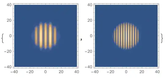
The results show

{DensityPlot[
  Evaluate[ Abs[\[Psi]1[0, x, y] /. solv[[1]]]], {x, -halfLx, 
   halfLx}, {y, -halfLy, halfLy}, PlotPoints -> 100, PlotRange -> All],
 DensityPlot[{Abs[Evaluate[initial\[Psi]1[x, y]]]}, {x, -halfLx, 
   halfLx}, {y, -halfLy, halfLy}, PlotPoints -> 100, 
  PlotRange -> All]}

Problem:

Obviously, the result given by NDsolve at t==0(left) is different from the initial state initial\[Psi]1[x, y](right).

I guess the reason is that the discretized space grid is too coarse, so it ignores the details therein. If the guess is correct, how can we control the size of the grid here? If not, what should we do?