This question is based on this answer
$Assumptions = {r ∈ Reals, r >= 0, rh ∈ Reals, rh > 0};
S[rh_] := π rh^2
M[rh_, qe_, qm_] =
  1/2 Sqrt[π/S[rh]] (S[rh]^2/π^2 + S[rh]/π + qe^2 + qm^2) // Simplify;
qe = SolveValues[ϕe == q (1/rh - 1/r), q][[1]] // Simplify;
f[r_, rh_, qm_, ϕe_] =
  1 + r^2/l^2 - (2 M[rh, qe, qm])/r + (qe^2 + qm^2)/r^2 // Simplify;
G[rh_, qm_, ϕe_] =
  1/(4 π^2) Sqrt[π/S[rh]] (3 π^2 qm^2 -
      S[rh]^2 + π S[rh] (1 - ϕe^2)) // Simplify;
T[rh_, qm_, ϕe_] = (-π^2 qm^2 +
      3 S[rh]^2 + π (S[rh] - S[rh] ϕe^2))/(4 (π S[rh])^(3/2)) //
   Simplify;
Veff[r_] = f[r, rh, qm, ϕe] (L^2/r^2 + 1) // FullSimplify;
eqn = L^2 == (r0^3 D[f[r0, rh, qm, ϕe], r0])/(2 f[r0, rh, qm, ϕe] -
        r0 D[f[r0, rh, qm, ϕe], r0]) /. r -> r0 // FullSimplify;
sol = Block[{l = 1, L = 20, ϕe = 3/5}, Solve[eqn, r0, Reals]];
l = 1; L = 20; ϕe = 3/5;
λ[rh_, qm_, ϕe_] =
  1/2 Sqrt[(r0 D[f[r0, rh, qm, ϕe], r0] - 2 f[r0, rh, qm, ϕe]) *
   Veff''[r0]] /. r -> r0 /. sol // Simplify;
Off[General::munfl, Less::nord]
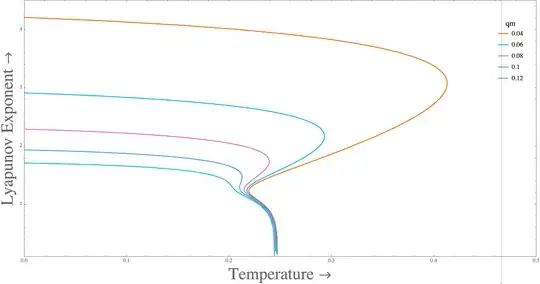
which I tried to generalize for multiple values of qm by using the standard method of creating a Table before plotting:
ParametricPlot[
 Evaluate@
  Table[{T[rh, qm, ϕe], #} & /@ (λ[rh,
       qm, ϕe][[{3, 5}]]), {qm, 0.04, 0.12, 0.02}], {rh, 0.01,
  8}, PlotRange -> {{0, 0.5}, {0.1, 4.5}}, AspectRatio -> 0.5,
 Exclusions -> All]
but unfortunately, it gives me a blank plot. Probably my use of a Table is erroneous when a map is being applied. Any help in this regard would be truly beneficial!

Tand other parameters, so we can run the code. It may also help if you remove the formatting niceties if they are not relevant to the problem. They just clutter the code up and may mask an otherwise obvious issue. – MarcoB May 04 '23 at 14:25