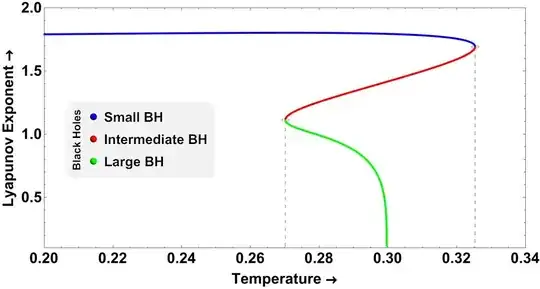
Color coding a parametric plot based on given conditions

Question

This question is based on the answers provided here and here. Basically, I have the following Mathematica code to calculate the Lyapunov exponents as a function of Temperature:

$Assumptions = {r \[Element] Reals, r >= 0, rh \[Element] Reals, 
   rh > 0};
S[rh_] := [Pi] rh^2
M[rh_, qe_, qm_] = 
  1/2 Sqrt[[Pi]/S[rh]] (S[rh]^2/[Pi]^2 + S[rh]/[Pi] + qe^2 + 
      qm^2) // Simplify;
qe = SolveValues[[Phi]e == q (1/rh - 1/r), q][[1]] // Simplify;
f[r_, rh_, qm_, [Phi]e_] = 
  1 + r^2/l^2 - (2 M[rh, qe, qm])/r + (qe^2 + qm^2)/r^2 // Simplify;
G[rh_, qm_, [Phi]e_] = 
  1/(4 [Pi]^2) Sqrt[[Pi]/S[rh]] (3 [Pi]^2 qm^2 - 
      S[rh]^2 + [Pi] S[rh] (1 - [Phi]e^2)) // Simplify;
T[rh_, qm_, [Phi]e_] = (-[Pi]^2 qm^2 + 
      3 S[rh]^2 + [Pi] (S[rh] - 
         S[rh] [Phi]e^2))/(4 ([Pi] S[rh])^(3/2)) // Simplify;
Veff[r_] = f[r, rh, qm, [Phi]e] (L^2/r^2 + 1) // FullSimplify;
eqn = L^2 == (r0^3 D[f[r0, rh, qm, [Phi]e], 
         r0])/(2 f[r0, rh, qm, [Phi]e] - 
        r0 D[f[r0, rh, qm, [Phi]e], r0]) /. r -> r0 // FullSimplify;
sol = Block[{l = 1, L = 20, [Phi]e = 3/5}, Solve[eqn, r0, Reals]];
l = 1; L = 20; [Phi]e = 3/5;
[Lambda][rh_, qm_, [Phi]e_] = 
  1/2 Sqrt[(r0 D[f[r0, rh, qm, [Phi]e], r0] - 
          2 f[r0, rh, qm, [Phi]e])*Veff''[r0]] /. r -> r0 /. sol // 
   Simplify;
Off[General::munfl, Less::nord]

I wished to colour-code the plot like one of my previous works as provided here:

for which I tweaked the original code to something like this:

qm = 0.05;
(tp1 = Evaluate[{#[[1]], #} & /@ (\[Lambda][rh1 = (rh /. #[[2]]), 
            qm, \[Phi]e][[{3, 5}]])] &@
      Maximize[{T[rh, qm, \[Phi]e], 0.01 < rh < 1}, rh] // 
     FullSimplify) // N;
(tp2 = Evaluate[{#[[1]], #} & /@ (\[Lambda][rh2 = (rh /. #[[2]]), 
            qm, \[Phi]e][[{3, 5}]])] &@
      Minimize[{T[rh, qm, \[Phi]e], rh1 < rh < 1}, rh] // 
     FullSimplify) // N;
pplt1 = ParametricPlot[
   Evaluate[{T[rh, 0.05, 0.6], #} & /@ ([Lambda][rh, 0.05, 
        0.6][[{3, 5}]])], {rh, 0.01, 2}, 
   PlotRange -> {{0, 0.4}, {0.1, 4}}, AspectRatio -> 0.5, 
   Exclusions -> All, PlotPoints -> 100, ImageSize -> 800, 
   PlotTheme -> {"Scientific", "NeonColor"}, 
   FrameLabel -> {"Temperature [Rule]", "Lyapunov Exponent [Rule]"},
    LabelStyle -> {Bold, Black, 22}, PlotStyle -> Thickness[0.004],
   ColorFunction -> 
    Function[{T, [Lambda], rh}, 
     If[rh <= rh1, Blue, If[rh <= rh2, Red, Green]]], 
   ColorFunctionScaling -> False,
Prolog -> {{Gray, Dashing[0.008], Line[{tp1, {tp1[[1]], 0}}], 
      Line[{tp2, {tp2[[1]], 0}}]}, {Gray, Thick, Dashing[0.001], 
      Circle[tp1, {0.005, .1}], Circle[tp2, {0.005, .1}]}}];
P1 = Legended[pplt1, 
  Placed[SwatchLegend[{Blue, Red, Green}, {"Small BH", 
     "Intermediate BH", "Large BH"}, LabelStyle -> {Bold, Black, 20}, 
    LegendMarkers -> "SphereBubble", LegendMarkerSize -> 20, 
    LegendFunction -> (Framed[#, RoundingRadius -> 10, 
        FrameStyle -> None, Background -> GrayLevel[0.95]] &), 
    LegendLabel -> 
     Placed["Black Holes", Left, 
      Rotate[Style[#, 16], 90 Degree] &]], {0.2, .45}]]

But it doesn't provide me with a colour-coded plot like the one I had previously and gives me this instead, along with lots of error messages:

score 2 · Answer 1 · answered May 06 '23 at 15:54

Changing only your last section of code.

qm = 1/20;
{max, arg} = 
  Maximize[{T[rh, qm, ϕe], 1/100 < rh < 1}, rh] // FullSimplify;
lambda = λ[rh1 = rh /. arg, qm, ϕe] // N
(* {0. + 2.07076 I, 31.6831, 2.52729, 0. + 1.92368 I, Undefined, Undefined} *)

Only the third value is applicable

tp1 = {max, lambda[[3]]};
{min, arg2} = 
  Minimize[{T[rh, qm, ϕe], rh1 < rh < 1}, rh] // FullSimplify;
lambda2 = λ[rh2 = rh /. arg2, qm, ϕe] // N
(* {0. + 2.25536 I, 8456.35, 1.23382, 0. + 1.63239 I, Undefined, Undefined} *)

Again, only the third value is applicable

tp2 = {min, lambda2[[3]]};
pplt1 = ParametricPlot[
  Evaluate[{T[rh, qm, ϕe], λ[rh, qm, ϕe][[3]]}],
  {rh, 0.01, 2},
  PlotRange -> {{0, 0.4}, {0.1, 4}},
  AspectRatio -> 0.5,
  Exclusions -> All,
  PlotPoints -> 100, 
  ImageSize -> 800,
  PlotTheme -> {"Scientific", "NeonColor"},
  FrameLabel -> {"Temperature [Rule]", "Lyapunov Exponent [Rule]"}, 
  LabelStyle -> {Bold, Black, 22},
  PlotStyle -> Thickness[0.004],
  ColorFunction -> Function[{T, λ, rh}, 
    If[rh <= rh1, Blue, If[rh <= rh2, Red, Green]]],
  ColorFunctionScaling -> False,
  Prolog -> {{Gray, Dashing[0.008], Line[{tp1, {tp1[[1]], 0}}], 
     Line[{tp2, {tp2[[1]], 0}}]}, {Gray, Thick, Dashing[0.001], 
     Circle[tp1, {0.005, .1}], Circle[tp2, {0.005, .1}]}}];
P1 = Legended[pplt1, Placed[
   SwatchLegend[
    {Blue, Red, Green}, {"Small BH", "Intermediate BH", "Large BH"},
    LabelStyle -> {Bold, Black, 20},
    LegendMarkers -> "SphereBubble",
    LegendMarkerSize -> 20,
    LegendFunction -> (Framed[#, RoundingRadius -> 10, 
        FrameStyle -> None, Background -> GrayLevel[0.95]] &),
    LegendLabel -> 
     Placed["Black Holes", Left, Rotate[Style[#, 16], 90 Degree] &]],
   {0.2, .45}]]

kglr · Accepted Answer · 2023-05-06T18:03:46.450

2

qm = 1/20;
ϕe = 3/5;

xc[rh_] := T[rh, qm, ϕe]
yc[rh_] := λ[rh, qm, ϕe][[3]]


colors = {Blue, Red, Green}; 

displayFunc = ReplaceAll[l_Line :> 
    {Last[colors = RotateLeft[colors]], l, Gray, Dashed, 
     Line[{#, {1, 0} #}] & /@ l[[1, {1, -1}]]}] @* Normal;

ParametricPlot[{xc @ rh, yc @ rh}, {rh, 0.01, 2},
 PlotRange -> {{0, 0.4}, {0.1, 4}},
 AspectRatio -> 0.5, MeshFunctions -> {xc'[#3] &}, 
 Mesh -> {{0}}, 
 MeshStyle -> PointSize[Large],
 MeshShading -> colors, 
 DisplayFunction -> displayFunc]

edited May 06 '23 at 18:03

answered May 06 '23 at 17:54

kglr

394,356
18
477
896

Ah, such a short code! I am new to the mesh functions. Can you explain a little about how are they used here to calculate the minima or maxima? It seems quite elegant to be honest. – codebpr May 07 '23 at 06:05
1

@codebpr, please see this answer by Silvia – kglr May 07 '23 at 14:54

Color coding a parametric plot based on given conditions

2 Answers2