Numerical integration of a list

Question

I have a list, p, obtained by a complex numerical procedure. Its element has the structure: {k,fi,z}. Below I give a simplified version of this list containing 36 elements. Here the step of k is 1 and the step of fi is 2Pi/5. In real calculation, the steps will be much smaller, and the list - much larger. So, here is an example:

 p= {{0., 0., 0.}, {0., 1.25664, 0.}, {0., 2.51327, 0.}, {0., 3.76991,0.}, {0., 5.02655, 0.}, {0., 6.28319, 0.}, {1., 0., 58.927}, {1., 
  1.25664, 1.02628}, {1., 2.51327, 28.3293}, {1., 3.76991, 
  28.3293}, {1., 5.02655, 1.02628}, {1., 6.28319, 58.927}, {2., 0., 
  3.06756}, {2., 1.25664, 0.134298}, {2., 2.51327, 1.63558}, {2., 
  3.76991, 1.63558}, {2., 5.02655, 0.134298}, {2., 6.28319, 
  3.06756}, {3., 0., 0.579411}, {3., 1.25664, 0.0616836}, {3., 
  2.51327, 0.355197}, {3., 3.76991, 0.355197}, {3., 5.02655, 
  0.0616836}, {3., 6.28319, 0.579411}, {4., 0., 0.194156}, {4., 
  1.25664, 0.0308556}, {4., 2.51327, 0.130682}, {4., 3.76991, 
  0.130682}, {4., 5.02655, 0.0308556}, {4., 6.28319, 0.194156}, {5., 
  0., 0.0879579}, {5., 1.25664, 0.0171569}, {5., 2.51327, 
  0.0618171}, {5., 3.76991, 0.0618171}, {5., 5.02655, 0.0171569}, {5.,
   6.28319, 0.0879579}};

I need to integrate the function z=z(k,fi) over its arguments: from 0 to infinity over k and from 0 to 2Pi over fi.

What I have done so far is the following:

f = Interpolation[p, InterpolationOrder -> 3];
int = NIntegrate[
  f[k, fi], {fi, 0, 2 \[Pi]}, {k, 0, 5}, 
  Method -> {"EvenOddSubdivision", Method -> "LocalAdaptive"}, 
  PrecisionGoal -> 6]

This approach works. My question is if there is a better one.

My question: Is there a built-in or workaround method in Mma, so I can make this numerical integration without passing to the interpolation function?

In other words, is there a method that enables one to integrate the list p directly without further intermediate actions numerically?

Answer 1

On the data:

The array p is given rounded to 6 sig. figs. (PrintPrecision), but the interval of integration for one of the variables is given as $[0,2\pi]$. I changed the Pi-based dimension (2nd coordinate) to have complete 15.95-digit machine precision. I could have changed the 2 Pi, which would have been easier; but I did it this way and didn't want to rework it. The first coordinate is an integer and correctly rounded to machine precision; it needs no fixing. I could not fix the 3rd coordinate, so that will make the results below different those computed from the OP's actual data.

The fixed 2nd coordinate:

p = p /. (N@Round[#, 10^-5] -> # & /@ (2. Pi Range[5]/5));

Several methods:

For interpolating over a rectangular grid, Integrate/InterpolatingFunction has a built-in method for integrating, which I assume integrates the polynomial interpolants and gives the most accurate result (how to test that hypothesis though?):

Integrate[f[x, y], x, y] /. 
  Thread[{x, y} -> f["Domain"][[All, 2]]] // RepeatedTiming
(*  {0.000202620849609375`, 156.39842883024124`}   *)

It is faster than the OP's method:

int = NIntegrate[f[k, fi], {fi, 0, 2 π}, {k, 0, 5}, 
   Method -> {"EvenOddSubdivision", Method -> "LocalAdaptive"}, 
   PrecisionGoal -> 6] // RepeatedTiming
(*  {0.0409303125`,         156.39869606089889`}    *)

Another built-in method is Method -> "InterpolationPointsSubdivision"", which is faster and gives the same answer as Integrate; it gives the exact same answer as the Automatic method but more slowly.

NIntegrate[f[k, fi], {fi, 0, 2 π}, {k, 0, 5}, 
  Method -> "InterpolationPointsSubdivision"] // RepeatedTiming
(*  {0.00022087890625`,     156.39842883024124`}  *)
NIntegrate[f[k, fi], {fi, 0, 2 π}, {k, 0, 5}] // RepeatedTiming
(*  {{0.0005922978515625, 156.39842883024124}  *)

A manual implementation of "InterpolationPointsSubdivision" gives the same answer as Integrate, but much more slowly:

NIntegrate[
  f[k, fi],
  Evaluate[
   Sequence @@ MapThread[Prepend, {f@"Coordinates", {k, fi}}]]
  ] // RepeatedTiming
(*  {0.0322208125`,         156.39842883024122`}  *)

Remark: Integrate[f[x, y], x, y] gives an interpolating function representing $\int_{y_1}^y \int_{x_1}^x f(x,y)\; dx\,dy$, which can be very useful.

---

Addendum: Trapezoidal without Interpolation[]

pp = Partition[p, 6];
fvals = pp[[All, All, 3]];
coords1 = pp[[All, 1, 1]];
coords2 = pp[[1, All, 2]];
Developer`PartitionMap[
  Mean@*Flatten, fvals,
  {2, 2}, {1, 1}
  ] . Differences@coords1 . Differences@coords2
(*  158.712  *)

Alternatively, for a uniformly spaced grid (as in the OP), using fvals above:

wts = ConstantArray[1., Dimensions@fvals];
wts[[All, 1]] /= 2;
wts[[All, -1]] /= 2;
wts[[1]] /= 2;
wts[[-1]] /= 2;
Total[wts*fvals, 2]*
 (pp[[2, 1, 1]] - pp[[1, 1, 1]])*
 (pp[[1, 2, 2]] - pp[[1, 1, 2]])
(*  158.712  *)

Addendum 2: Simpson's without Interpolation[]

Need Dimensions@fvals to both be odd, or the last interval will be chopped off. Since the OP's p is a 6 x 6 array (of three coordinates), the following underestimates the integral. The grid also needs to be uniformly spaced.

Total[
  Developer`PartitionMap[
   # . {1, 4, 1} . {1, 4, 1}/36 &, fvals,
   {3, 3}, {2, 2}
   ],
  2] *
 (pp[[3, 1, 1]] - pp[[1, 1, 1]]) *
 (pp[[1, 3, 2]] - pp[[1, 1, 2]])

Answer 2

I think we need to use Interpolation and it is recommend to use InterpolationOrder -> 0.

We compare with the two cases.

Clear[data];
SeedRandom[1];
data = RandomReal[{-2, 1}, {10, 3}];

• InterpolationOrder -> 0

{ListPlot3D[data, InterpolationOrder -> 0, PlotStyle -> Opacity[.8], 
   Filling -> Bottom, Mesh -> All, PlotRange -> All, 
   FillingStyle -> Cyan], 
  ListPointPlot3D[data, PlotStyle -> {AbsolutePointSize[8], White}]} //
  Show[#, Background -> Black, ViewPoint -> Top, 
   ViewProjection -> "Orthographic"] &

When we use InterpolationOrder -> 0, the domain will be subdivided by the VoronoiMesh method.

• InterpolationOrder -> 1

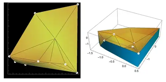
{ListPlot3D[data, InterpolationOrder -> 1, PlotStyle -> Opacity[.8], 
   Filling -> Bottom, Mesh -> All, PlotRange -> All, 
   FillingStyle -> Cyan], 
  ListPointPlot3D[data, PlotStyle -> {AbsolutePointSize[8], White}]} //
  Show[#, Background -> Black, ViewPoint -> Top, 
   ViewProjection -> "Orthographic"] &

When we use InterpolationOrder -> 1, the domain will be subdivided by the DelaunayMesh method and construct a convex region which contain all the points and there are many point on the boundary.