Filling a curve to a vertical axis: Q#2

Question

I found an elegant solution to my problem on this site in the answer No 2 to the post Filling a curve to a vertical axis. Consider the following example:

lst = Table[{1.3 - Sin[\[Pi] t], 1.4 - Cos[\[Pi] t]}, {t, 0, 1, 0.05}];
lst2 = Table[{1.5 - 0.8 Sin[[Pi] t], 1.9 - 0.3 Cos[[Pi] t]}, {t, 0, 
    1, 0.05}];
plt = ListLinePlot[{lst, lst2}, Joined -> True, 
  PlotMarkers -> Automatic
  , AxesOrigin -> {0, 0}]

It yields

Applying to this plot function

fillVertical[plot_, x0_ : 0.] := 
  plot /. Line[
     p_] :> {{Opacity[0.2], 
      Polygon[p~Join~{{N@x0, p[[-1, 2]]}, {N@x0, p[[1, 2]]}}]}, 
     Line[p]};

as proposed in Filling a curve to a vertical axis gives almost what I need:

fillVertical[plt, 0.1]

To become even more happy, I would like to have an option. e.g., to switch off vertical filling for second, third, e.t.c. curves, i.e., for lst2 in the example above. Second desired option is to extend filing to the bottom and to the top of the picture. My knowledge of Wolfram Language is insufficient to find how I could do that.

Update

Please note that I need a solution which would preserve style of plot markers and correct plot legends.

kglr · Accepted Answer · 2023-07-28T12:46:46.727

ClearAll[addHorizontalFilling]

addHorizontalFilling[pos_ : All, pr_ : Automatic] := 
  Module[{xyr = pr /. Automatic -> 
      Transpose @ Charting`get2DPlotRange[If[Head @ # === Legended, First@#, #]],
    xyrnp = pr /. Automatic -> 
      Transpose @ PlotRange[If[Head @ # === Legended, First @ #, #]]},
    xyr = {Clip[#, First @ xyrnp], #2} & @@ xyr;
    ReplaceAt[#, l_Line :>
      Module[{cl = Transpose[{Clip[#, First @ Transpose @ xyr], 
             Clip[#2, Last @ Transpose @ xyr]} & @@ Transpose[l[[1]]]]}, 
       {l, Opacity[.2], 
        Polygon[Join[{xyr[[1]], {cl[[1, 1]], xyr[[1, 2]]}}, cl, 
         {{0, xyr[[2, 2]]} + {cl[[-1, 1]], 0}, {xyr[[1, 1]], xyr[[2, 2]]}}]]}], 
      Position[#, _Line][[pos]]]] &;

Examples:

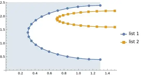
llp = ListLinePlot[{lst, lst2}, Joined -> True, 
   PlotMarkers -> Automatic, AxesOrigin -> {0, 0}, 
   PlotLegends -> {"list 1", "list 2"}];

Add horizontal filling to all curves (default):

addHorizontalFilling[] @ llp

Add filling to the first curve only:

addHorizontalFilling[1] @ llp

Add filling to the second curve only:

addHorizontalFilling[2] @ llp

Use the second argument to specify the rectangle coordinates to be filled:

addHorizontalFilling[All, {{.1, .5}, {1.2, 2.2}}] @ llp

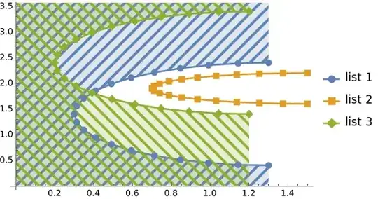
Add filling to curves 1 and 3:

pltb = addHorizontalFilling[{1, 3}] @
 ListLinePlot[{lst, lst2, Threaded[{-.1, 1}] + lst}, 
  Joined -> True, 
  PlotMarkers -> Automatic, 
  AxesOrigin -> {0, 0}, 
  PlotLegends -> {"list 1", "list 2", "list 3"}, 
  PlotRange -> {{0, All}, {0, All}}]

hatchFillings = HatchFilling[#, 2, 10] & /@ {Pi/4, -Pi/4, Pi};
ReplaceAll[{l_Line, a___, p_Polygon} :>
   {l, a, p, Opacity[1],
    Last[hatchFillings = RotateLeft[hatchFillings]], p}] @ pltb

Solution of @kglr is excellent from all points of view. Unfortunately, it assumes that option PlotRangeClipping is set to False which is not my case. Therefore, currently I am using a hybrid of solutions proposed by @kglr and @DanielHuber. Is there a method to put some text outside PlotRange without setting PlotRangeClipping to False? Or to impose some window for filling? — Igor Kotelnikov, Jul 20 '23 at 01:27
I accepted your answer. Thank you so much. Nevertheless, at the moment I am using my own solution which is less difficult to understand. I'll post my answer soon. — Igor Kotelnikov, Jul 23 '23 at 14:00
It seems that this method fails in Mathematica 13.2 for plots without PlotLegeds, get2DPlotRange[If[Head @ # == Legended, First@#, #]] does not work as expected. — Igor Kotelnikov, Jul 28 '23 at 11:16
@IgorKotelnikov, thank you for the catch. I fixed the problem (Head @ # == Legended should be Head @ # === Legended ) — kglr, Jul 28 '23 at 12:48

score 3 · Answer 2 · answered Jul 18 '23 at 11:55

To apply filling only to the first curve, you make a plot of the first curve with filling and a second plot withoutfilling of the rest of the curves and show them together:

lst1 = Table[{1.3 - Sin[\[Pi] t], 1.4 - Cos[\[Pi] t]}, {t, 0, 1, 
    0.05}];
lst2 = Table[{1.5 - 0.8 Sin[\[Pi] t], 1.9 - 0.3 Cos[\[Pi] t]}, {t, 0, 
    1, 0.05}];
pl1 = ListLinePlot[{lst1}, Joined -> True, PlotMarkers -> Automatic, 
   AxesOrigin -> {0, 0}];
pl2 = ListLinePlot[{lst2}, Joined -> True, PlotMarkers -> Automatic, 
   AxesOrigin -> {0, 0}];
fillVertical[plot_, x0_ : 0.] := 
  plot /. Line[
     p_] :> {{Opacity[0.2], 
      Polygon[p~Join~{{N@x0, p[[-1, 2]]}, {N@x0, p[[1, 2]]}}]}, 
     Line[p]};
Show[fillVertical[pl1, 0.1], pl2]

To make filling to the bottom and top, you must split the data so that the function is unique. Then you plot the lower part with filling to the bottom and the upper part with filling to the top:

lst11 = Table[{1.3 - Sin[\[Pi] t], 1.4 - Cos[\[Pi] t]}, {t, 0, 1/2, 
    0.05}];
lst12 = Table[{1.3 - Sin[\[Pi] t], 1.4 - Cos[\[Pi] t]}, {t, 1/2, 1, 
    0.05}];
pl11 = ListLinePlot[{lst11}, Joined -> True, PlotMarkers -> Automatic,
    AxesOrigin -> {0, 0}, Filling -> Bottom];
pl12 = ListLinePlot[{lst12}, Joined -> True, PlotMarkers -> Automatic,
    AxesOrigin -> {0, 0}, Filling -> Top];
Show[{pl11, pl12}, PlotRange -> All]

This is not what i want. I have used separate filling for upper and lower branches in the past. I want a better solution which would keep style of markers and correct plot legends. I'll update my question. — Igor Kotelnikov, Jul 18 '23 at 13:30

Igor Kotelnikov · Answer 3 · 2023-07-23T23:26:08.807

I accepted solution by @kglr although still use my own version:

fillVertical6[plt_, pos_ : All] := Module[{x0, x1, y0, y1}
  ,
  {{x0, x1}, {y0, y1}} = 
   Charting`get2DPlotRange[
    If[Head@# == Legended, First@#, #] &[plt]];
  (*Print[];*)
  ReplaceAt[#, l_Line :> {l, Opacity[.25]
       , Polygon[Join[
         {{x0, y0},
            {x1, y0}, {x1, #[[2]]}} &@( l[[1, 1]])
         , {{x1, #[[2]]}} &@( l[[1, 1]])
         , l[[1]]
         , {#, {x1, #[[2]]}, {x1, y1}, {x0, y1}} &@(l[[1, -1]])]]}, 
     Position[#, _Line][[pos]]] &[plt]
  ]
lst = Table[{1.3 - Sin[[Pi] t], 1.4 - Cos[[Pi] t]}, {t, 0, 1, 0.05}];
lst2 = Table[{1.5 - 0.8 Sin[[Pi] t], 1.9 - 0.3 Cos[[Pi] t]}, {t, 0, 
    0.7, 0.05}];
plt = ListLinePlot[{lst, lst2, Threaded[{-.1, 1}] + lst}, 
  Joined -> True, PlotMarkers -> Automatic, PlotLegends -> Automatic
  , PlotRange -> {{0.1, Full}, {0, Full}}
  , Prolog -> {Text[Style["lbl", Blue, 16], 
     Scaled[{0.5, 1.04}], {0, 1}]}
  , PlotRangeClipping -> False]
fillVertical6[plt, {1, 3}]

This is a bit different from @kglt's solution:

ClearAll[addHorizontalFilling]
addHorizontalFilling[pos_ : All, pr_ : Automatic] := 
  Module[{xyr = 
      pr /. Automatic -> 
        Transpose@
         Charting`get2DPlotRange[If[Head@# == Legended, First@#, #]], 
     xyrnp = pr /. 
       Automatic -> 
        Transpose@PlotRange[If[Head@# == Legended, First@#, #]]}, 
    xyr = {Clip[#, First@xyrnp], #2} & @@ xyr;
    ReplaceAt[#, 
     l_Line :> 
      Module[{cl = 
         Transpose[{Clip[#, First@Transpose@xyr], 
             Clip[#2, Last@Transpose@xyr]} & @@ 
           Transpose[l[[1]]]]}, {l, Opacity[.2], 
        Polygon[Join[{xyr[[1]], {cl[[1, 1]], xyr[[1, 2]]}}, 
          cl, {{0, xyr[[2, 2]]} + {cl[[-1, 1]], 0}, {xyr[[1, 1]], 
            xyr[[2, 2]]}}]]}], Position[#, _Line][[pos]]]] &;
addHorizontalFilling[{1, 3}]@plt

Filling a curve to a vertical axis: Q#2

3 Answers3