I am trying to improve the numerical solution of some PDEs that develop a piecewise behavior during their evolution. The simplest example of one such PDE is for a function $u(t,x)$ with $t \in [-T,T]$ and $x \in \mathbb{R}$: $$u_t(t,x) = \frac{\sqrt{T^2-t^2}}{2\pi T^2} \frac{t^2 f(x) u_{xx}(t,x)}{1- t u_x(t,x)},$$ with initial condition $u(-T,x) = f(x)$ and boundary conditions $u(t,x) \sim f(x)$ for large $|x|$, implemented numerically by choosing a value $L$ and imposing $u(t,\pm L) = f(\pm L)$. For the examples here I will focus on $f(x) = {\rm LogisticSigmoid}(x) = 1/(1+\exp(-x))$.
The behavior of the solution depends on the value of the parameter $T$, which sets the initial and final "time". For sufficiently small $T$ the solution remains smooth, but for sufficiently large $T$ I expect there will be a time $t_\ast$ and point $x_\ast$ such that $1 - t_\ast u_x(t_\ast,x_\ast) = 0$--i.e., the denominator vanishes, but I also expect this will be compensated by $u_{xx}(t_\ast,x_\ast) = 0$. The solution can continue for $t_\ast < t$ if it becomes piecewise linear, such that there is a range $x^-(t) < x < x^+(t)$ for which $1 - t u_x(t,x) = u_{xx}(t,x) = 0$, and otherwise obeys the above PDE when $x$ is outside this range.
I have solved the above PDE numerically using two methods. The first is NDSolve using MethodOfLines with a TensorProductGrid discretization:
mineg[T_, L_] :=
 NDSolve[{D[u[t, x], t] ==
    Sqrt[T^2 - t^2]/(2*Pi*T^2)*t^2*LogisticSigmoid[x]*
     D[u[t, x], x, x]/(1 - t*D[u[t, x], x]),
   u[-T, x] == LogisticSigmoid[x], u[t, -L] == LogisticSigmoid[-L],
   u[t, L] == LogisticSigmoid[L]}, u, {t, -T, T}, {x, -L, L},
  Method -> {"PDEDiscretization" -> {"MethodOfLines",
      "SpatialDiscretization" -> {"TensorProductGrid",
        "MinPoints" -> {600}}}}]
egT10L40 = mineg[10, 40]
(* Plot solution versus initial condition *)
Manipulate[
 Plot[{LogisticSigmoid[x], Evaluate[u[t, x] /. egT10L40]}, {x, -10,
   10}, PlotRange -> {0, 1}], {t, -10, 10}]
(* Plot denominator to see that it runs up against zero )
Manipulate[
 Plot[{1 - tLogisticSigmoid'[x],
   Evaluate[1 - t*Derivative[0, 1][u][t, x] /. egT10L40]}, {x, -10,
   10}, PlotRange -> {-4, 4}], {t, -10, 10}]
(* Plot second derivative *)
Manipulate[
 Plot[{LogisticSigmoid''[x],
   Evaluate[Derivative[0, 2][u][t, x] /. egT10L40]}, {x, -10, 10},
  PlotRange -> {-0.25, 0.25}], {t, -10, 10}]
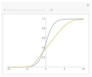
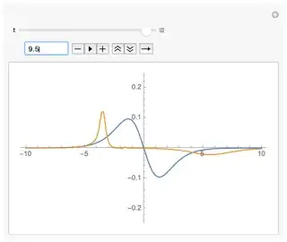
You can see that as $t$ runs from $-T$ to $T$ the solution eventually reaches a point where the denominator appears to touch zero, and then continues to be pressed against zero instead of becoming negative, and in this region the second derivative is also close to zero. The behavior gets a bit noisy as $t$ approaches $T$, and while this qualitatively agrees with the picture I claimed above, I am not sure if there is any artifact coming from the numerator and denominator both approaching zero numerically.
Solution at $t = T = 10$, compared to initial condition.
Denominator at $t = 10$ (compared to a fictitious denominator with the initial condition plugged in)
Second derivative at $t = 10$. Note the sharp peak near $x = -5$.
I attempted to improve this numerical solution by using the pdetoode tool developed by @xzczd:
Tp = 10; Lp = 40;
eqn = D[u[t, x], t] ==
   Sqrt[Tp^2 - t^2]/(2*Pi*Tp^2)*t^2*LogisticSigmoid[x]*
    D[u[t, x], x, x]/(1 - t*D[u[t, x], x]);
ic = {u[-Tp, x] == LogisticSigmoid[x]};
bc = {u[t, -Lp] == LogisticSigmoid[-Lp],
   u[t, Lp] == LogisticSigmoid[Lp]};
(Difference order of x:)
xdifforder = 4;
points = 500;
grid = Array[# &, points, {-Lp, Lp}];
(There're 2 b.c.s,so we need to remove 2 equations from every

PDE/i.c.,usually the difference equations that are the "closest" ones

to the b.c.s are to be removed:)
removeredundant = #[[2 ;; -2]] &;
(Use pdetoode to generate a "function" that discretizes the spatial

derivatives of PDE(s) and corresponding i.c.(s) and b.c.(s):)
ptoofunc = pdetoode[u[t, x], t, grid, xdifforder];
odeqn = eqn // ptoofunc // removeredundant;
odeic = removeredundant /@ ptoofunc@ic;
odebc = bc // ptoofunc;
sollst = NDSolveValue[{odebc, odeic, odeqn}, u /@ grid, {t, -Tp, Tp},
   MaxSteps -> Infinity];
(Rebuild the solution for the PDE from the solution for the ODE set:)
sol = rebuild[sollst, grid];
(* Solution compared to initial condition *)
Manipulate[
 Plot[{LogisticSigmoid[x], sol[t, x]}, {x, -10, 10},
  PlotRange -> All], {t, -Tp, Tp}]
(* Denominators )
Manipulate[
 Plot[{1 - tLogisticSigmoid'[x],
   1 - t*Derivative[0, 1][sol][t, x]}, {x, -10, 10},
  PlotRange -> {-4, 4}], {t, -Tp, Tp}]
(* Second derivatives *)
Manipulate[
 Plot[{LogisticSigmoid''[x], Derivative[0, 2][sol][t, x]}, {x, -10,
   10}, PlotRange -> {-0.25, 0.25}], {t, -Tp, Tp}]
Solution at $t = 10$
Denominator:
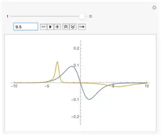
Second derivative:
This appears to improve the stability of the solution, can go to larger values of $T$, and maintains the qualitative picture I described where it appears that the solution is becoming close to piecewise linear in the center. However, it does not appear to have as flat a region as I would expect, and attempts to find zero crossings numerically only return a single value. This value also does not coincide with the point where the solution appears to abruptly become exactly equal to the initial condition for negative $x$ (roughly near -4 or -5).
Perhaps this is a limitation of the method of solution, but I am wondering if the solution can be improved further to actually implement the piecewise linear behavior by identifying when the denominator vanishes and then imposing that at later times the solution is linear between edges $x^-(t)$ and $x^+(t)$ that move in time and must also be tracked. This sounds superficially similar to problems on this site solving PDEs with Stefan boundary conditions, though these boundaries appear inside the solution at some intermediate time $t_\ast$.
Specific issues/questions:
I imagine that to do this I would need to first identify when ($t_\ast$) and where ($x_\ast$) the denominator vanishes, and then track the evolution of the boundary points for times $t_\ast < t$. I know WhenEvent does not work on bivariate functions; I imagine something can be done with the pdetoode discretization, but I am not sure how to implement it.
I am not sure how to derive equations that dictate the evolution of the piecewise linear region boundary points $x^\pm(t)$. I would have guessed that I would define these points by $1 - t u_x(t,x^\pm(t)) = 0$ and differentiate this relationship, but it did not appear to give me something useful. This also does not seem to be how the boundary conditions are derived in the Stefan boundary problems I saw in other questions (e.g., here.). I am not clear on whether the moving boundaries in those questions are just given as part of the model/problem statement, or if there is a way to derive differential equations for moving boundaries from the governing differential equation for the full solution and the definition of the boundary.
Any help figuring out how to improve the numerical solution will be much appreciated.


