Simulating buckling

Question

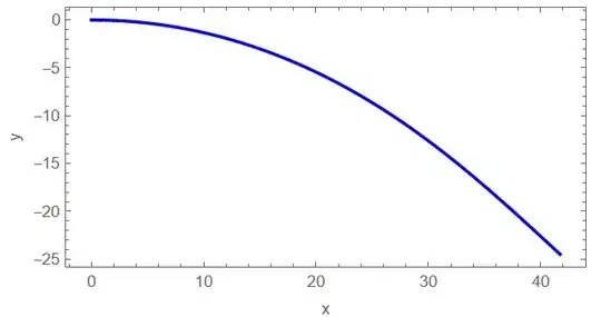
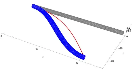
We are trying to implement buckling using a newly implemented FEM solver. However, if we try to reproduce the buckling phenomena using a thin rod, it is just compressed, and we cannot observe the buckling phenomenon. It may be due to the absence of small noise in the shape of the rod, but we are not sure how to implement this phenomenon. The code we use is attached below.

Needs["NDSolve`FEM`"];
length = 50;
radius = 1;
YoungModulus = 260000;
PoissonRatio = 0.3;
MassDensity = 1300;
Pressure = -1 100000 ;
MaxCellMeasureLength = radius/4;
vars = {{u[x, y, z], v[x, y, z], w[x, y, z]}, {x, y, z}}; pars = <|
  "YoungModulus" -> YoungModulus , "PoissonRatio" -> PoissonRatio, 
  "MassDensity" -> MassDensity|>;
op1 = SolidMechanicsPDEComponent[vars, pars];
[CapitalOmega] = Cylinder[{{0, 0, 0}, {0, 0, length}}, radius];
mesh = ToElementMesh[[CapitalOmega] , MeshQualityGoal -> 1, 
   MaxCellMeasure -> {"Length" -> MaxCellMeasureLength}];
Subscript[[CapitalGamma], load] = 
  SolidBoundaryLoadValue[ElementMarker == 2, vars, 
   pars, <|"Pressure" -> Pressure {0, 0, 1}|>];
Subscript[[CapitalGamma], base] = 
  SolidDisplacementCondition[ElementMarker == 3, vars, 
   pars, <|"Displacement" -> {0, 0, 0}|>];
pde = {op1 == Subscript[[CapitalGamma], load], 
   Subscript[[CapitalGamma], base]};
measure = 
  AbsoluteTiming[
   MaxMemoryUsed[
     displacement = 
      NDSolveValue[
       pde, {u[x, y, z], v[x, y, z], 
        w[x, y, z]}, {x, y, z} [Element] mesh]
     ]/(1024.^2)];
Print["Time -> ", measure[[1]], "\nMemory -> ", measure[[2]]];
visualizeDeformation[fun : {__InterpolatingFunction}, 
   OptionsPattern[]] := 
  Module[{mesh}, mesh = fun[[1]]["ElementMesh"];
   Show[{mesh["Wireframe"["MeshElement" -> "BoundaryElements"]], 
     ElementMeshDeformation[mesh, fun, "ScalingFactor" -> 1
       ][
      "Wireframe"[
       "ElementMeshDirective" -> 
        Directive[EdgeForm[Red], FaceForm[]]]]}, Axes -> True]];
visualizeDeformation[displacement[[All, 0]]]

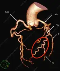
2023/12/4 Thank you very much for all the comments - they are all informative. But I think I need to clarify why I need the slight shape deviation. I am dealing with interdigitation of blood vessels caused by blood pressure or vessel growth to a longitudinal direction, which seems to have a certain characteristic length. My main interest is where this length comes from.

I started from the linear theory to predict initial growth of pattern as we usually do in other PDE. Euler-Bernoulli beam theory is

0 = -P h''(x) - EI h''''(x)

where P is the pressure caused by growth, and EI is Young's modulus times inertia. This describes the balance of force from pressure and force from elasticity, so if we assume the viscosity-dominant condition in which growth is slow and the growth of the deviation is proportional to the force, the dynamic version of the equation becomes

Then by the linear stability analysis we can obtain

which seem to match the numerical simulation result.

L = 6.28;
EI = 1;
P = 25;
simulationLength = 10;
dx = 0.2;
dt = 0.0001;
nStep = 100;
loopPerStep = Round[simulationLength/dt/nStep];
n = Round[L/dx];
h0 = Table[0.01 (RandomReal[] - 0.5), {n}];
dd[l_] := (RotateLeft[l] + RotateRight[l] - 2 l)/dx/dx;
dhdt[h_] := h + dt (-P dd[h] - EI dd[dd[h]]);
oneStep[h_] := Nest[dhdt, h0, loopPerStep];
result = NestList[oneStep, h0, nStep];
{ Sqrt[P/(2 EI)] // N, ListLinePlot[result[[2]]]}

I am curious whether we could obtain similar winding pattern using FEM simulation. I am not sure whether I can get this by simply changing the pressure direction, and still want to know how to introduce slight shape deviation (in this case h0 = Table[0.01 (RandomReal[] - 0.5), {n}];)

Thank you very much in advance.

Answer 1

We have already discussed this issue once here. Due to large deformations of the thin beam in a case of buckling we need probably some nonlinear model. As is known, in the case of a cylinder, loss of stability is observed under load $F=\pi^2 Y I/4 l^2$, where $I=\pi r^4/4$, $r$ is a radius, $l$ is a length of cylinder. In a discussed case we have

length = 50;
radius = 1;
YoungModulus = 260000;inert = Pi radius^4/4; F=Pi^2 Y inert/4/length^2 // N 
(*201.541*) 

Thus, if the load is greater than 201.541 Newton, then loss of stability will be observed. The final shape of the rod can be calculated using thin rod theory, for example

Pressure = -70; 
L = length; Y = YoungModulus; fX = 
 Pi radius^2 (-Pressure);
q[t0_] := 
 Sqrt[1/2 inert Y/fX] 2 Sqrt[1/(1 - Cos[t0])]
   EllipticF[t0/2, Csc[t0/2]^2]
t0 = t /. NSolve[q[t] - L == 0 && 0 <= t <= Pi, t, Reals][[1]]
(Out[]= 0.827734)

Using parameter t0 we can compute coordinate of the rod in parametric form as follows

yl[t_] := -Sqrt[2 inert Y/fX] (Sqrt[1 - Cos[t0]] - 
     Sqrt[Cos[t] - Cos[t0]]);
xl[t_?NumericQ] := 
  Sqrt[.5 inert Y/fX] NIntegrate[
    Cos[tet]/Sqrt[Cos[tet] - Cos[t0]], {tet, 0, t}];
ParametricPlot[{xl[t], yl[t]}, {t, 0, t0}, PlotRange -> All, 
  FrameLabel -> {"x", "y"}, PlotStyle -> Blue, Frame -> True, 
  AspectRatio -> 1/2]

This is the shape the cylinder should take in the event of loss of stability. We can use this data in a 3D linear model. To do this, we calculate the deformation of the end of the rod as follows

final = {xl[t0] - L, yl[t0], 0}
Out[]= {-8.26458, -24.5092, 0}

In the example we are considering, the load is carried out along the x-axis.

Needs["NDSolve`FEM`"];
length = 50;
radius = 1;
YoungModulus = 260000;
PoissonRatio = 0.3;
MassDensity = 1300;
Pressure = -70;
MaxCellMeasureLength = radius/4;
vars = {{u[x, y, z], v[x, y, z], w[x, y, z]}, {x, y, z}}; pars = <|
  "YoungModulus" -> YoungModulus, "PoissonRatio" -> PoissonRatio, 
  "MassDensity" -> MassDensity|>;
op1 = SolidMechanicsPDEComponent[vars, pars];
[CapitalOmega] = Cylinder[{{0, 0, 0}, {length, 0, 0}}, radius];
mesh = ToElementMesh[[CapitalOmega], MeshQualityGoal -> 1, 
   MaxCellMeasure -> {"Length" -> MaxCellMeasureLength}];
Subscript[[CapitalGamma], load] = 
  SolidBoundaryLoadValue[x == length, vars, 
   pars, <|"Force" -> fX {1, 0, 0}|>];
Subscript[[CapitalGamma], 
   base] = {SolidFixedCondition[x == 0, vars, pars], 
   SolidDisplacementCondition[x == length, vars, 
    pars, <|"Displacement" -> final|>]};
pde = {op1 == Subscript[[CapitalGamma], load], 
   Subscript[[CapitalGamma], base]};
{U, V, W} = NDSolveValue[pde, {u, v, w}, {x, y, z} [Element] mesh]

Visualization

Show[{ElementMeshDeformation[mesh, {U, V, W}, "ScalingFactor" -> 1][
   "Wireframe"[
    "ElementMeshDirective" -> Directive[EdgeForm[Blue], FaceForm[]]]],
   mesh["Wireframe"["MeshElementStyle" -> EdgeForm[Gray]]], 
  ParametricPlot3D[{xl[t], yl[t], 0}, {t, 0, t0}, PlotRange -> All, 
   PlotStyle -> Red, AspectRatio -> 1/2]}, Axes -> True, 
 AxesLabel -> {x, y, z}]

We see that the cylinder does not take the shape of a thin rod.

Answer 2

This is not an answer but are the pieces I gather from the comments on how this should be done. But something is wrong and that's too much to discuss in a comment. So here it goes:

Set up:

Needs["NDSolve`FEM`"];
length = 50;
radius = 1;
YoungModulus = 260000;
PoissonRatio = 3/10;
(MassDensity=1300;)
vars = {{u[x, y, z], v[x, y, z], w[x, y, z]}, {x, y, z}}; pars = <|
  "YoungModulus" -> YoungModulus, "PoissonRatio" -> PoissonRatio|>;
op1 = SolidMechanicsPDEComponent[vars, pars];
region = Cylinder[{{0, 0, 0}, {0, 0, length}}, radius];
mesh = ToElementMesh[region];

Extract assemble the system matrices:

(* no rigid body modes should be present *)
{dPDE, dBCs, vd, sd, md} = 
  NDSolve`FEM`ProcessPDEEquations[{op1 == 
     SolidBoundaryLoadValue[z == length, vars, 
      pars, <|"Pressure" -> {0, 0, -1}|>], 
    SolidDisplacementCondition[z == 0, vars, 
     pars, <|"Displacement" -> {0, 0, 0}|>]}, {u[x, y, z], v[x, y, z],
     w[x, y, z]}, {x, y, z} \[Element] mesh];

Get the matrices:

{loadV, stiffnessM, dampingM, massM} = dPDE["SystemMatrices"];

Apply the boundary conditions:

DeployBoundaryConditions[{loadV, stiffnessM}, dBCs]

Compute the eigenvalue:

Eigenvalues[stiffnessM, -1, Method -> "Arnoldi"]
(* {0.00069054} *)

(And as requested in a comment, the first 20 eigenvalues, with this method)

Reverse[Eigenvalues[stiffnessM, -20, Method -> "Arnoldi"]]
(* {0.00069054, 0.000690565, 0.0266785, 0.0266805, 0.205952, 0.205977, 0.384391, 0.77103, 0.771207, 1., 1., 1., 1., 1., 1., 1., 1.39559, 2.02578, 2.02638, 3.46523} *)

Now, when we compare this to theory, (that Alex provided) we have:

inert = Pi  radius^4/4
(* pinned on one end *)
k = 2;
F = Pi^2  pars["YoungModulus"]  inert/(k*length)^2;
F//N
(* 201.541 *)

Something is wrong here. The one thing that confuses me is that the load actually does not play a role in this.

Update 1: In place of the force I now used a forced displacement:

(* no rigid body modes should be present *)
{dPDE, dBCs, vd, sd, md} = 
  NDSolve`FEM`ProcessPDEEquations[{op1 == {0, 0, 0}, 
    SolidDisplacementCondition[z == length, vars, 
     pars, <|"Displacement" -> {None, None, -1}|>], 
    SolidDisplacementCondition[z == 0, vars, 
     pars, <|"Displacement" -> {0, 0, 0}|>]}, {u[x, y, z], v[x, y, z],
     w[x, y, z]}, {x, y, z} \[Element] mesh];

The rest is the same and then I get an eigenvalue of:

Eigenvalues[stiffnessM, -1, Method -> "Arnoldi"]
(* {0.00174763} *)

Still no cookies :-(

Update 2: In place of the pressure I used a force:

{dPDE, dBCs, vd, sd, md} = 
  NDSolve`FEM`ProcessPDEEquations[{op1 == 
     SolidBoundaryLoadValue[z == length, vars, 
      pars, <|"Force" -> {0, 0, -1}|>], 
    SolidDisplacementCondition[z == 0, vars, 
     pars, <|"Displacement" -> {0, 0, 0}|>]}, {u[x, y, z], v[x, y, z],
     w[x, y, z]}, {x, y, z} \[Element] mesh];

Rest is the same, then we have:

Eigenvalues[stiffnessM, -1, Method -> "Arnoldi"]
{0.00069}