Curvature of a Klein bottle

Question

1. Problem statement

An old answer of mine: Computing Gaussian curvature shows how to color parametric curves and surfaces according to their curvature. However, the methods used there will fail for non-differentiable and very complicated functions. A workaround, not perfect, but the only one I know, is to color such surfaces according to their polygon sizes. Polygon areas decrease in zones of high curvature. I know how to use this "area method" in my Blender/Python application, but don't know how to transfer it to Mathematica.

2. Curvature of a Torus (formula method)

GaussianCurvature[f_] :=
 With[{dfu = D[f, u], dfv = D[f, v]}, 
  Simplify[(Det[{D[dfu, u], dfu, dfv}] * Det[{D[dfv, v], dfu, dfv}] - 
      Det[{D[f, u, v], dfu, dfv}]^2) / (dfu.dfu * dfv.dfv - (dfu.dfv)^2)^2]]
torus = {(2 + Cos[v]) Cos[u], (2 + Cos[v]) Sin[u], Sin[v]};
curvature = GaussianCurvature[torus]

Cos[v] / (2 + Cos[v])

range = Last[PlotRange /. AbsoluteOptions[Plot3D[curvature, {u, 0, 2 Pi}, {v, 0, 2 Pi}], PlotRange]]

{-1., 0.333333}

Legended[
 ParametricPlot3D[torus, {u, 0, 2 Pi}, {v, 0, 2 Pi},
  ColorFunction ->
   Function[{x, y, z, u, v},ColorData["TemperatureMap"][Rescale[curvature, range]]],
  ColorFunctionScaling -> False,
  ImageSize -> 400,
  Mesh -> False,
  PlotPoints -> 70],
 BarLegend[{"TemperatureMap", range}, Automatic]]

3. Curvature of a Torus with Blender/Python (area method)

The Blender 3.6.5 Python API has a method, calc_area() which returns a list of polygon sizes (basically with one line of code):

p.list = [f.calc_area() for f in bm.faces]

("Faces" are rectangular polygons defined by 4 points). A rescaled list of these sizes is then used to index the color table and color the polygons. We can see that the Blender result is very similar to the above Mathematica plot:

4. The Klein bottle

KleinBottle[u_, v_] :=
 Module[{a, b, c, x, y, z},
  a = 6 Cos[u] (1 + Sin[u]);
  b = 16 Sin[u];
  c = 5 (1 - Cos[u]/2);
  x = If[Pi < u <= 2 Pi, a + c Cos[v + Pi], a + c Cos[u] Cos[v]];
  y = If[Pi < u <= 2 Pi, b, b + c Sin[u] Cos[v]];
  z = c Sin[v];
  {x, y, z}]
klein =
 ParametricPlot3D[
  KleinBottle[u, v], {u, 0, 2 Pi}, {v, 0, 2 Pi},
  PlotPoints -> 60]

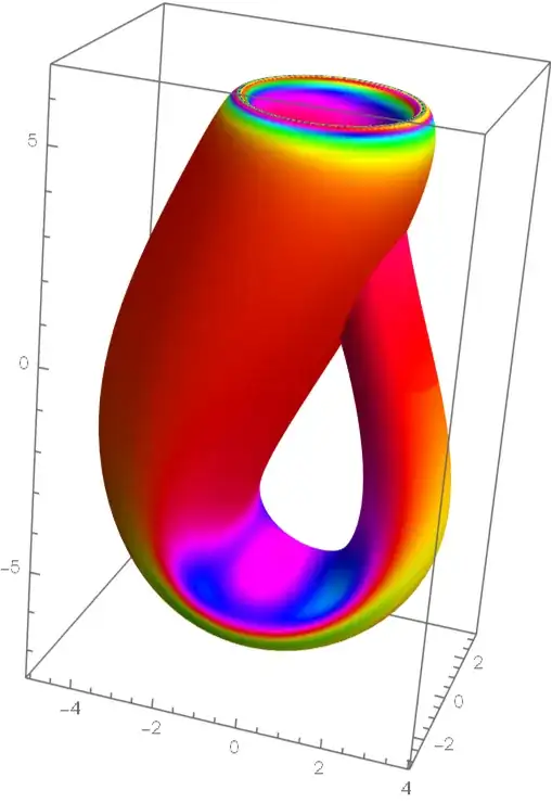
Because it is not possible to apply the curvature formula to this complicated surface, I show how it would look like in Blender using the "polygon area method" with a logarithmic scale and TemperatureMap imported from Mathematica:

5. Question

I know how to extract the polygons, f.e. the first polygon of the Klein bottle:

Cases[Normal[klein], _Polygon, Infinity][[1]] // PolygonCoordinates

{{8.80683, 0.984612, 0.133244}, {9.10008, 1.96794, 2.67745*10^-7}, {9.08591, 1.96642, 0.267239}}

But I don't know how to proceed from there to calculate the polygon sizes and color the bottle similar to the last screenshot.

Answer 1

Here one way to create a ParametricPlot3D of the Klein bottle with curvature dependent coloring:

First I take a smooth definition found on Wikipedia

kleinFlasche[u_, v_] := Block[{b = 2, h = 6, r = 2 - Cos[u]},
x = b (1 - Sin[u]) Cos[u] + r Cos[v] (2 Exp[-(u/2 - Pi)^2] - 1);
y = r Sin[v];
z = h Sin[u] + 1/2 r Sin[u] Cos[v] Exp[-(u - 3 Pi/2)^2];
{x, y, z}
]

curvature (Thanks to @eldo ;-) )

GaussCurvature[f_] := 
With[{dfu = D[f, u],dfv = D[f,v]}, 
(Det[{D[dfu, u], dfu, dfv}] Det[{D[dfv, v], dfu, dfv}] - 
Det[{D[f, u, v], dfu, dfv}]^2)
/(dfu . dfu dfv . dfv - (dfu . dfv)^2)^2] ;

Plot of the bottle

ParametricPlot3D[kleinFlasche[u, v], {u, 0, 2 Pi}, {v, 0, 2 Pi},
ColorFunctionScaling -> False, 
ColorFunction ->Function[{x, y, z, u,v},Evaluate[Hue[GaussCurvature[kleinFlasche[u, v]]]]], Mesh -> False,PlotPoints -> 100]

Hope it helps!

Answer 2

As a footnote to Ulrich Neumann's answer I would like to show how the bottle looks like with ColorData["TemperatureMap"]

curvature = GaussCurvature[kleinFlasche[u, v]];

The resulting function is too long to be shown here.

range =
 Last[PlotRange /. 
   AbsoluteOptions[Plot3D[curvature, {u, 0, 2 Pi}, {v, 0, 2 Pi}], PlotRange]]

{-0.580809, 0.504683}

Legended[
 ParametricPlot3D[kleinFlasche[u, v], {u, 0, 2 Pi}, {v, 0, 2 Pi},
  ColorFunction ->
   Function[{x, y, z, u, v},
    ColorData["TemperatureMap"][Rescale[curvature, range]]],
  ColorFunctionScaling -> False,
  ImageSize -> 400,
  Mesh -> False,
  PlotPoints -> 70],
 BarLegend[{"TemperatureMap", range}, Automatic]]

The output nicely shows the jump from positive to negative curvature at the top of the bottle.

Answer 3

The two cases of the embeddes surfaces have the line elements

  Collect[(# . # &)[Assuming[u < \[Pi],Simplify[
   du D[KleinBottle[u, v], u] + dv D[KleinBottle[u, v], v]]]] // 
FullSimplify // TrigReduce, {du, dv}] // Simplify

$$\frac{25}{16} \left(\text{du}^2 (\cos (2 (u-v))+\cos (2 (u+v))-4 \cos (u+2 v)-4 \cos (u-2 v)-8 \cos (u)+8 \cos (2 v)+10)-4 \text{du} \text{dv} \sin (u) (\cos (u)-2) \sin (2 v)+4 \text{dv}^2 (\cos (u)-2)^2\right)$$

Collect[(# . # &)[
 Assuming[2 \[Pi] > u > \[Pi], 
  Simplify[
   du D[KleinBottle[u, v], u] + dv D[KleinBottle[u, v], v]]]] // 
FullSimplify // TrigReduce, {du, dv}] // Simplify

$$\frac{25}{32} \left(8 \text{du}^2 \sin ^2(u) \sin ^2(v)-8 \text{du} \text{dv} \sin (u) (\cos (u)-2) \sin (2 v)+8 \text{dv}^2 (\cos (u)-2)^2\right)$$

Its not too difficult to obtain the curvature.