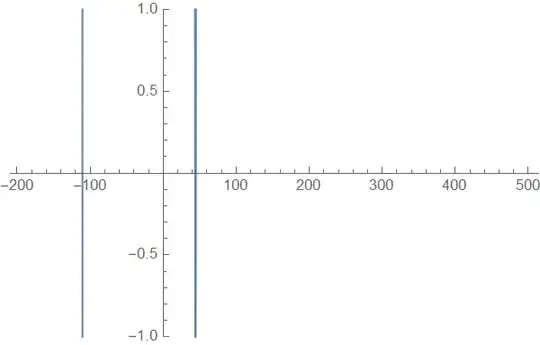
Solving A System of Two Implicit Equations

Question

I am solving a system of 6 equations, and I am interested to know the solution for different rhoBar values. Here is the input parameters:

(*Input Parameters*)
kB = 1.380649*10^-23; 
absTemp = 298.15;
beta = 1/(kB*absTemp);
eps0 = 8.8541878128*10^(-12);
eps = 78.6; 
f = 96485.33212;
e = 1.60217663*10^(-19);
nA = 6.02214076*10^(23);
u2 = -8/beta;
u1 = -8/beta;
u3 = -8/beta;
vW = 30*10^(-30);
vB = 5*10^(-30);
vD = 32*10^(-30);
vBnb = 5*vBb;
vBb = 30*10^(-30);
vCb = 100*10^(-30);
dLayBb = 250*10^(-12);
dLayBnb = 250*10^(-12);
dLayCb = 250*10^(-12);
k0 = 10^(-6.8)*nA;
pSite = 4.8*10^18;
cToBRatio = 0;
dToBRatio = 2;
c = -3;
rhoBar = 1.823348001*nA/dToBRatio;

The equations are:

eqn1Squared = (beta*e^2)/(
    2*rhoBar*eps*eps0)*(-2*pBnb - 2*pBb + pC + pSiO)^2 ==(*(10^(-8)*
   nA^2)/(dToBRatio*rhoBar^2) Exp[beta*(-e*phi0 +vD*
   osmP0)]*)+Exp[beta*(-2*e*phi0 - vB*osmP0)] + 
    cToBRatio*Exp[beta*(e*phi0 - vC*osmP0)] + 
    dToBRatio*Exp[beta*(e*phi0 - vD*osmP0)] + c;
eqn2 = pSiO == 
   pSite*(k0*dToBRatio*rhoBar*Exp[beta*(e*phi0 - vD*osmP0)])/(
    10^(-8)*nA^2 + 
     k0*dToBRatio*rhoBar*Exp[beta*(e*phi0 - vD*osmP0)]);
eqn3 = (pBnb - pC)/(pSiO - pBnb - 2*pBb) == 
   Exp[-beta*(u1 + 2*e*phi0 + osmP0*vBnb)];
eqn4 = (Sqrt[2]*pBb)/(pSiO - pBnb - 2*pBb) == 
   Exp[-0.5*beta*(u3 + 2*e*phi0 + osmP0*vBb)];
eqn5 = pC/(pBnb - pC) == Exp[beta*(u1 - u2 + e*phi0 - osmP0*vCb)];
eqn6 = 1 - pBb*vBb/dLayBb - pBnb*vBnb/dLayBnb - pC*vCb/dLayCb - 
    rhoBar*Exp[beta*(-2*e*phi0 - vB*osmP0)]*vB - 
    cToBRatio*rhoBar*Exp[beta*(e*phi0 - vC*osmP0)]*vC - 
    dToBRatio*rhoBar*Exp[beta*(e*phi0 - vD*osmP0)]*
     vD == (1 - rhoBar*vB - cToBRatio*rhoBar*vC - 
      dToBRatio*rhoBar*vD)*Exp[-beta*vW*osmP0];

Solving eqn2, eqn3, eqn4, eqn5, I managed to decouple the system of 6 equations into system of 2 equations, with variable phi0 and osmP0 left to be solved.

solution2345 = Solve[{eqn2, eqn3, eqn4, eqn5}, {pSiO, pBnb, pBb, pC}];

I then substitute solutions from eqn2 to eqn5 into eqn1Squared and eqn6

eqn1Squared = eqn1Squared /. solution2345[[1]];
eqn1Squared = eqn1Squared /. {osmP0 -> osmP0*10^6};
eqn1Squared = eqn1Squared /. {phi0 -> phi0*10^-3};
funcPhi0[phi0_, osmP0_] = (eqn1Squared[[1]] - eqn1Squared[[2]]);
eqn6 = eqn6 /. solution2345[[1]];
eqn6 = eqn6 /. {osmP0 -> osmP010^6};
eqn6 = eqn6 /. {phi0 -> phi010^-3};
funcOsmP0[phi0_, osmP0_] = (eqn6[[1]] - eqn6[[2]]);

I had tried NSolve the solve eqn6 and eqn1Squared. This did not work as it took forever to run. Then, I tried FindRoot. This method is not very reliable as I had to input guessed values for phi0 and osmP0 everytime I change the input parameter, rhoBar. To know the guessed values, I had to visually inspect the intersection between eqn6 and eqn1Squared using ContourPlot:

plot = ContourPlot[{funcPhi0[phi0, osmP0] == 0, 
   funcOsmP0[phi0, osmP0] == 0}, {phi0, -200, 500}, {osmP0, -2000, 
   2000}, MaxRecursion -> 4, PlotPoints -> 75]

I am now thinking to convert eqn6 (or its function funcOsmP0==0) into an interpolating function, osmP0 that is expressed as a function of phi0. This is so that I could substitute the function of osmP0 into eqn1Squared and solve it easily. I came across this post, and its solution could only turn the multi-line contour plot into a parametric curve.

My questions are:

How can I adapt its solution into my problem, and convert the implicit equation plotted in ContourPlot (f(x,y)=0) into a one to one function, or even into a one to many function (As a simple example: f(x,y)=x^2+y^2=4)?
Is there a more reliable and straightforward method to solve my problem? I want to solve my system of equations for various combination of input parameters, hence I am aiming to find an automated solving procedure.

Are you looking for the intersectionpoints in your plot? – Ulrich Neumann Nov 11 '23 at 21:26 — Ulrich Neumann, Nov 11 '23 at 21:26

Ulrich Neumann · Accepted Answer · 2023-11-12T09:28:28.570

First plot the function you want tointerpolate

plot2 = ContourPlot[ funcOsmP0[phi0, osmP0] == 0 , {phi0, -200, 500},{osmP0, -2000, 2000}, MaxRecursion -> 4, PlotPoints -> 75]

interpolation of plotted points

pts2=plot2[[1, 1]][[1]];
ip2 = Interpolation[pts2]
Plot[funcPhi0[phi0, ip2[phi0] ] , {phi0, ip2["Domain"][[1, 1]], 
ip2["Domain"][[1, 2]]}, PlotRange -> {-1 , 1 }]

Plot shows zeros near phi0=44 and phi0=-110

NMinimize[{funcPhi0[phi0, ip2[phi0] ]^2, phi0 > 44}, phi0 ]
(*{1.93291*10^-27, {phi0 -> 44.6898}}*)
NMinimize[{funcPhi0[phi0, ip2[phi0] ]^2, phi0 < 44 }, phi0 ]
({6.4929510^-14, {phi0 -> 43.6525}}*)
NMinimize[{funcPhi0[phi0, ip2[phi0] ]^2, -120 < phi0 < -100 }, phi0 ]
({5.695510^-23, {phi0 -> -110.572}}*)

Hope it helps!

addendum

Without "guessing" the phi0 try

zero1 = NMinimize[{funcPhi0[phi0, ip2[phi0]]^2 }, phi0]
(*{8.17923*10^-26, {phi0 -> 44.6898}}*)
max1 = NMaximize[{(funcPhi0[phi0, ip2[phi0]]/(phi0 - (phi0 /. zero1[[2]])))^2,ip2["Domain"][[1, 1]] < phi0 < ip2["Domain"][[1, 2]]},phi0]
zero2 = NMinimize[1/max1[[1]] ( funcPhi0[phi0, ip2[phi0]]/(phi0 - (phi0 /. zero1[[2]])))^2  , phi0]
({7.2620110^-19, {phi0 -> 43.6525}}*)
max2 = NMaximize[{(funcPhi0[phi0,ip2[phi0]]/((phi0 - (phi0 /.zero1[[2]])) (phi0 - (phi0 /. zero2[[2]]))))^2,ip2["Domain"][[1, 1]] < phi0 < ip2["Domain"][[1, 2]]}, phi0]
zero3 = NMinimize[1/max2[[1]] (funcPhi0[phi0,ip2[phi0]]/((phi0 -(phi0 /. zero1[[2]])) (phi0 - (phi0 /.zero2[[2]]))))^2  , phi0]
({1.1437110^-34, {phi0 -> -110.572}}*)

Stop iterated search if minimum found takes finite value !=0

Thanks!, is there a way to solve for phi0 without requiring guessed input? — Johnson, Nov 12 '23 at 08:20

bbgodfrey · Answer 2 · 2023-11-12T17:02:15.057

An alternative approach is to use FindRoot or FindMinimum without constructing an InterpolatimgFunction, if rough estimates of the desired solutions can be provided.

FindRoot[{funcPhi0[phi0, osmP0], funcOsmP0[phi0, osmP0]}, {{phi0, -100}, {osmP0, 100}}]
(* {phi0 -> -110.572, osmP0 -> 89.7373} *)
FindMinimum[{(funcPhi0[phi0, osmP0] - funcOsmP0[phi0, osmP0])^2, 
    funcPhi0[phi0, osmP0] == 0, funcOsmP0[phi0, osmP0] == 0}, 
    {{phi0, -100}, {osmP0, 100}}]
(* {2.5769310^-15, {phi0 -> -110.572, osmP0 -> 89.7373}} )
FindRoot[{funcPhi0[phi0, osmP0], funcOsmP0[phi0, osmP0]}, {{phi0, 50}, {osmP0, 150}}]
(* {phi0 -> 44.8119, osmP0 -> 124.638} *)
FindMinimum[{(funcPhi0[phi0, osmP0] - funcOsmP0[phi0, osmP0])^2, 
    funcPhi0[phi0, osmP0] == 0, funcOsmP0[phi0, osmP0] == 0}, 
    {{phi0, 50}, {osmP0, 150}}]
(* {2.6266710^-21, {phi0 -> 44.8119, osmP0 -> 124.638}} )
FindRoot[{funcPhi0[phi0, osmP0], funcOsmP0[phi0, osmP0]}, {{phi0, 40}, {osmP0, 120}}]
(* {phi0 -> 43.7612, osmP0 -> 125.286} *)
FindMinimum[{(funcPhi0[phi0, osmP0] - funcOsmP0[phi0, osmP0])^2, 
    funcPhi0[phi0, osmP0] == 0, funcOsmP0[phi0, osmP0] == 0}, 
    {{phi0, 40}, {osmP0, 120}}]
(* {2.9101810^-22, {phi0 -> 43.7612, osmP0 -> 125.286}} )

Results are identical to about ten significant figures. Which of FindRoot and FindMinimum is preferable depends on details of the problem to be solved.

Solving A System of Two Implicit Equations

2 Answers2