How can we reproduce Otti Bergers winding carpet patterns?

Question

Otti Berger was a textile designer and weaver of Jewish heritage. She was born in Zmajevac (Austro-Hungarian Empire, present day Croatia) in 1898. Berger attended the Bauhaus school between 1926 and 1930, where she became a close friend of Anni Albers, who I introduced in another post:

How to weave Anni Albers Red Meander carpet?

In 1931 Otti Berger began teaching at Bauhaus at the recommendation of weaving director Gunta Stölzl. She left there in 1932 and set up her own design business in Berlin. Legislation passed in 1936 banned Jewish people from having business in Germany. Berger was forced into exile, going to London whilst awaiting an American visa. But due to the ill-health of her mother she returned to Croatia. This return tragically resulted in her deportation to Auschwitz concentration camp, where she was murdered in 1944.

Posthumously, her works were and are shown in renowned museums around the world, including the MoMA.

Carpet 1

Her beautiful carpet shown above somehow reminded me of a Lissajous figure. In that era, many artists were fascinated by mathematical structures and objects, including Bergers artist colleague Max Ernst. Ernst actually used a Harmonograph to sketch his "Non-Euclidean Fly".

Max Ernst, Young Man Intrigued by the Flight of a Non-Euclidean Fly, 1942

Max Ernst making Lissajous figures, New York, 1942

One of my first reproduction trials is at best an approximation of Otti Bergers wavy structures:

ParametricPlot[{Sin[1.798 t + 1.89124], Sin[1.0 t]}, {t, 0, 80},
 AspectRatio -> 1.25,
 Axes -> False,
 Background -> RGBColor[0.75,0.3,0.2]
 PlotRangePadding -> None,
 PlotStyle -> Lighter @ Gray]

The injection of some randomness doesn't help too much either:

 ParametricPlot[{Sin[0.9 t + 0.2] Cos[0.502 t], Sin[0.2 t + 0.8] Cos[0.2 t]}, {t, 0, 120},
 AspectRatio -> 1.25,
 Axes -> False,
 Background -> RGBColor[0.75,0.3,0.2]
 PlotRangePadding -> None,
 PlotStyle -> Lighter @ Gray]

Carpet 2

Another Otti Berger rug that I really like is this one:

Here, my approximation uses an adaption of Alfred Gray's intrinsic function (Alfred Gray, Modern differential geometry of curves and surfaces with Mathematica, -- 3rd ed., Boca Raton 2006, p 140 ff)

intrinsic[f_, a_, r_][t_] :=
 Module[{x, y, p, s, sol},
  sol =
   {x'[s] == Cos[p @ s], y'[s] == Sin[p @ s], p'[s] == f[s],
    x[0] == 0, y[0] == 0, p[0] == a};
  sol = NDSolve[sol, {x, y, p}, {s, -r, r}];
  {x[t], y[t]} /. sol[[1]]]
r = 30;
ParametricPlot[
 Evaluate[intrinsic[# Cos[0.24 #] &, 5, r][t]], {t, -r, r},
 AspectRatio -> 1.25,
 Axes -> False,
 Background -> RGBColor[0.7, 0.6, 0.3, 0.5],
 ColorFunction -> "RedBlueTones",
 GridLines -> {Range[-2, 2, 0.2], Range[-2, 2, 0.2]},
 GridLinesStyle -> Directive[RGBColor[0.7, 0.6, 1, 0.5], Thickness[0.001]],
 PlotPoints -> 100,
 PlotRangePadding -> None,
 PlotStyle -> Directive[Lighter @ Gray, Thickness[0.04]]]

Question

How can we get closer to Otti Bergers weaving patterns?

Regarding the first carpet, I think that a GridGraph based solution could be a much better alternative, and for the second I don't have any idea if and how it can be improved.

Addendum

I just found an interesting article about pentagonal weaving patterns in the Journal of Mathematics and the Arts which might be helpful in finding a graph-based solution:

Answer 1

• For a curve we try to construct a polygon as its dilation.
• For such polygon we use WindingPolygon with "TwoRule" to find its self intersection parts.
• After that we use WhenEvent to look for the time which the line go through such region.

ρ[t_] = {6 Cos[t] - 3 Cos[6 t], 6 Sin[t] - 3 Sin[6 t]};
plot = ParametricPlot[ρ[t] + 
    s*Normalize[
      RotationMatrix[π/2] . ρ'[t], # . #/Sqrt[# . #] &], {t, 
    0, 2 π}, {s, -1, 1}, PlotStyle -> None, PlotPoints -> 50, 
   MaxRecursion -> 2];
regs = WindingPolygon[
   MeshPrimitives[DiscretizeGraphics@plot, 1][[;; , 1]][[;; , 1]], 
   "TwoRule"];
regs = MeshPrimitives[regs, 2];
dists = SignedRegionDistance /@ regs;
n = Length@regs;
fig[c_] := 
 Module[{r, sols, pic, above, below}, 
  r[t_] := ρ[t] + 
    c*Normalize[
      RotationMatrix[π/2] . ρ'[t], # . #/Sqrt[# . #] &];
  sols = 
   Table[Reap@
     NDSolve[{z'[t] == r'[t], z[0] == r[0], 
       WhenEvent[dists[[i]]@z[t] == 0, Sow[t]]}, 
      z, {t, 0, 2 π}], {i, 1, n}];
  pic = Table[
    ParametricPlot[z[t] /. sols[[1, 1, 1]], {t, 0, 2 π}, 
     RegionFunction -> 
      Function[{x, y, t}, 
       And @@ Table[! (sols[[i, 2, 1, 1]] <= t <= sols[[i, 2, 1, 2]] ||
             sols[[i, 2, 1, 3]] <= t <= sols[[i, 2, 1, 4]]), {i, 1, 
          n}]]], {i, 1, n}];
  above = 
   Table[ParametricPlot[z[t] /. sols[[1, 1, 1]], {t, 0, 2 π}, 
     RegionFunction -> 
      Function[{x, y, t}, 
       sols[[i, 2, 1, 1]] <= t <= sols[[i, 2, 1, 2]]]], {i, 1, n}];
  below = 
   Table[ParametricPlot[z[t] /. sols[[1, 1, 1]], {t, 0, 2 π}, 
     RegionFunction -> 
      Function[{x, y, t}, 
       sols[[i, 2, 1, 3]] <= t <= sols[[i, 2, 1, 4]]]], {i, 1, n}];
  {pic, above, below}]

choice = RandomChoice[{1, -1}, n]
Show[Table[{fig[c][[1,1]], 
   fig[c][[2]][[Position[choice, 1] // Flatten]], 
   fig[c][[3]][[Position[choice, -1] // Flatten]]}, {c,Subdivide[-.9, .9, 4]}],
  Axes -> False, Frame -> False, PlotRange -> All]

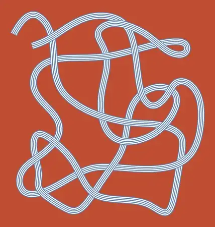
• The above method work when the curve not so sharp and does not overlay so much.

Clear["Global`*"];
Charting`$InteractiveHighlighting = False;
pts = {{0, 0}, {1, 1}, {2, -1}, {3, 0}, {4, -2}, {6, 1}, {2, 3}, {2, 
    0}, {3, -2}, {4, -1}, {5, 2}, {4, 2}, {3, 2}, {1, 1}, {1, -1}};
ρ = BSplineFunction[pts];
L = .12;
s[t_] = ρ[t] + 
   c*Normalize[
     RotationMatrix[π/2] . ρ'[t], # . #/Sqrt[# . #] &];
{a, b} = {0, 1};
plot = ParametricPlot[s[t], {t, a, b}, {c, -L, L}, PlotStyle -> None, 
   PlotPoints -> 60, MaxRecursion -> 2, PlotRange -> All];
regs = MeshPrimitives[
   WindingPolygon[
    MeshPrimitives[DiscretizeGraphics@plot, 1][[;; , 1]][[;; , 1]], 
    "TwoRule"], 2];
dists = SignedRegionDistance /@ regs;
n = Length@regs;
m = 5;
data = Table[
   Reap@NDSolve[{z'[t] == s'[t], z[a] == s[a], 
      WhenEvent[dists[[i]]@z[t] == 0, Sow[t]]}, z, {t, a, b}, 
     MaxStepSize -> 10^-3 L], {i, 1, n}, {c, 
    Subdivide[-.8 L, .8 L, m - 1]}];
fig0 = Show[
   Table[ParametricPlot[
     z[t] /. data[[1, j, 1]] // Evaluate, {t, 0, 1}, 
     MeshStyle -> Transparent, 
     Mesh -> {Sort@Flatten@Table[data[[i, j, 2]], {i, 1, n}]}, 
     MeshShading -> {Automatic, None}], {j, 1, m}], Axes -> False];

belt = ParametricPlot[s[t], {t, 0, 1}, {c, -.8 L, .8 L}, Mesh -> None,
    PlotStyle -> Directive[Opacity[1], White], BoundaryStyle -> None, 
   PlotPoints -> 80, MaxRecursion -> 2];
trans = Table[
   RandomChoice[{SubsetMap[Reverse, {2, 4}], Identity}], {i, 1, n}];
fig = Table[
    ParametricPlot[z[t] /. data[[i, j, 1]] // Evaluate, {t, 0, 1}, 
     Mesh -> data[[i, j, 2]], MeshStyle -> Transparent, 
     MeshShading -> 
      trans[[i]]@{None, Automatic, None, None, None}], {i, 1, n}, {j, 
     1, m}] // Show;
Show[belt, fig0, fig, Axes -> None, Frame -> None, 
 Background -> RGBColor[0.75, 0.3, 0.2]]

• We can use Canvas[] to draw a line and extract the points from it by img[[1, 1]][[1 ;; -1 ;; 50]].

pts = {{-0.8833333333333332`, 
    0.6901204427083333`}, {-0.7785346137152778`, 
    0.8880995008680556`}, {-0.6285346137152777`, 
    0.8603217230902778`}, {-0.5313123914930555`, 
    0.6547661675347222`}, {-0.5368679470486111`, 
    0.3825439453125`}, {-0.48409016927083337`, 
    0.1964328342013888`}, {-0.3368679470486111`, 
    0.07421061197916656`}, {-0.20075683593750004`, 
    0.004766167534722143`}, {-0.04242350260416661`, \
-0.04801161024305567`}, {0.16313205295138888`, \
-0.08690049913194442`}, {0.3409098307291667`, -0.08412272135416665`}, \
{0.4825764973958333`, -0.12023383246527786`}, {0.6075764973958333`, \
-0.1952338324652778`}, {0.5659098307291668`, -0.4007893880208333`}, \
{0.5214653862847223`, -0.6896782769097223`}, {0.46868760850694446`, \
-0.9119004991319444`}, {0.3075764973958335`, -0.7813449435763888`}, \
{0.16868760850694442`, -0.7507893880208334`}, \
{-0.014645724826388928`, -0.7424560546875001`}, \
{-0.17853461371527768`, -0.720233832465278`}, {-0.27853461371527777`, \
-0.5924560546875`}, {-0.35909016927083326`, -0.40634494357638884`}, \
{-0.4924235026041667`, -0.2674560546875`}, {-0.6618679470486111`, \
-0.1424560546875`}, {-0.7202012803819444`, -0.2230116102430555`}, \
{-0.7007568359375`, -0.3646782769097223`}, {-0.6479790581597222`, \
-0.5146782769097222`}, {-0.6896457248263889`, -0.6369004991319445`}, \
{-0.6007568359375`, -0.720233832465278`}, {-0.4535346137152778`, \
-0.8146782769097225`}, {-0.311867947048611`, -0.8813449435763889`}, \
{-0.14797905815972223`, -0.6285671657986112`}, \
{-0.045201280381944375`, -0.47856716579861125`}, \
{0.06590983072916679`, -0.33412272135416665`}, {0.10202094184027777`, \
-0.13690049913194446`}, {0.12979871961805567`, 
    0.0714328342013888`}, {0.24646538628472237`, 
    0.20198838975694433`}, {0.39924316406250004`, 
    0.2492106119791666`}, {0.5409098307291667`, 
    0.19087727864583326`}, {0.5464653862847222`, 
    0.05198838975694442`}, {0.388132052951389`, \
-0.1785671657986112`}, {0.08257649739583339`, -0.27856716579861107`}, \
{-0.10909016927083326`, -0.1591227213541666`}, {-0.1424235026041667`, 
    0.15476616753472228`}, {-0.04797905815972214`, 
    0.4269883897569444`}, {-0.10353461371527772`, 
    0.5964328342013889`}, {-0.18686794704861098`, 
    0.7075439453125`}, {-0.028534613715277768`, 
    0.8214328342013889`}, {0.28257649739583335`, 
    0.7075439453125`}, {0.4547987196180556`, 
    0.5158772786458333`}, {0.635354275173611`, 
    0.49643283420138884`}, {0.6381320529513888`, 
    0.6492106119791666`}, {0.3492431640625`, 
    0.6103217230902778`}, {-0.08409016927083335`, 
    0.4714328342013888`}, {-0.4368679470486111`, 
    0.49643283420138884`}, {-0.6674235026041666`, 
    0.4380995008680555`}, {-0.7396457248263889`, 
    0.25476616753472214`}, {-0.6535346137152778`, 
    0.11032172309027777`}, {-0.4979790581597222`, \
-0.025789388020833304`}, {-0.4618679470486111`, \
-0.1869004991319445`}, {-0.6202012803819444`, -0.3507893880208335`}, \
{-0.8063123914930556`, -0.4563449435763889`}, {-0.8535346137152777`, \
-0.6035671657986112`}, {-0.7702012803819445`, -0.731344943576389`}, \
{-0.5313123914930555`, -0.6480116102430555`}, {-0.2757568359375`, \
-0.47856716579861125`}, {-0.09520128038194442`, \
-0.45078938802083335`}, {0.18257649739583348`, -0.4841227213541668`}, \
{0.5020209418402779`, -0.47856716579861125`}, {0.6909098307291668`, \
-0.35356716579861125`}, {0.7547987196180554`, -0.10912272135416679`}, \
{0.7492431640624999`, 0.15754394531250004`}, {0.6297987196180554`, 
    0.29087727864583335`}, {0.5103542751736112`, 
    0.28254394531249993`}, {0.4575764973958334`, 
    0.14921061197916674`}, {0.33535427517361116`, 
    0.03532172309027781`}, {0.2159098307291667`, 
    0.1325439453124999`}, {0.18813205295138902`, 
    0.4658772786458333`}, {0.1436876085069445`, 
    0.7130995008680555`}, {0.049243164062499956`, 
    0.8214328342013889`}, {-0.09520128038194442`, 
    0.8575439453125`}, {-0.2563123914930556`, 
    0.8408772786458334`}, {-0.43964572482638886`, 
    0.7436550564236111`}, {-0.6035346137152777`, 
    0.6214328342013888`}, {-0.7229790581597222`, 
    0.5880995008680555`}};

and set L = .035;, we get

• For Lissajous curve.

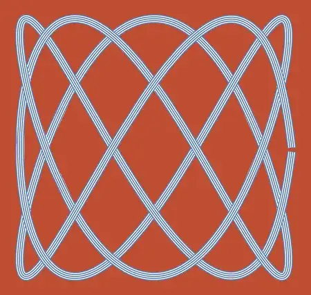
pts = Table[{Cos[3 t], Sin[5 t]}, {t, Subdivide[0, .999*2 π, 50]}];
ρ = BSplineFunction[pts];
L = .035;

Answer 2

It is far from ideal nevertheless I am sharing it.

po = {{0, 0}, {1, 1}, {0, 2}, {-1, 1}, {0, 0}};
pts = Flatten[
   Table[(#*{1, (-1)^n} + {2 n, 0}) & /@ ((1 + 
         Mod[Floor[n/2], 2]) po), {n, 0, 10}], 1];
pts = (Append[#, 0] & /@ pts) + 
   Flatten[Table[Append[Table[{0, 0, 0}, 4], {0, 0, 1}], 11], 1];
Graphics3D[{Tube[BSplineCurve[pts], 0.3, 
   VertexColors -> 
    RotateRight[
     Join @@ Table[Join @@ #, 3] &@
      RandomSample[{Table[Red, 5], Table[Cyan, 5], Table[Blue, 5], 
        Table[Yellow, 5]}]]]}, ViewProjection -> "Orthographic", 
 ViewPoint -> {0, 0, 2}, ViewVertical -> {0, 1, 0}, 
 Lighting -> "ThreePoint", Boxed -> False]

po = {{0, 0}, {1, 1}, {0, 2}, {-1, 1}, {0, 0}};
pts = Flatten[
   Table[(#*{1, (-1)^n} + {2 n, 0}) & /@ ((1 + 
         Mod[Floor[n/2], 2]) po), {n, 0, 10}], 1];
pts = (Append[#, 0] & /@ pts) + 
   Flatten[Table[Append[Table[{0, 0, 0}, 4], {0, 0, 1}], 11], 1];
Graphics3D[{Thickness[
   0.03], (d |-> 
     Line[((-1)^(d[[2]]/8) + 1) {-10.5, 0, 0} + (-1)^(
          d[[2]]/8)*#*{1, (-1)^(d[[2]]/8), 1} + d & /@ pts, 
      VertexColors -> 
       RotateRight[
        Join @@ Table[Join @@ #, 3] &@
         RotateRight[
          SequenceReplace[
           RandomChoice[{Table[Lighter@Lighter@Red, 5], 
             Table[Lighter@Red, 5], Table[Lighter@Lighter@Blue, 5], 
             Table[Lighter@Blue, 5]}, 30], {Repeated[a_, Infinity]} :>
             a], RandomInteger[10]], (-1)^(d[[2]]/8)]]) /@ 
   Table[{0, 8 n, 0}, {n, 0, 2}]}, ViewProjection -> "Orthographic", 
 ViewPoint -> {0, 0, 2}, ViewVertical -> {0, 1, 0}, 
 Lighting -> "ThreePoint", Boxed -> False, 
 Background -> RGBColor[0.9, 0.8, 0.5], 
 FaceGrids -> {{{0, 0, -1}, {Range[-100, 100, 1]}, 
    Range[-100, 100, 1]}}]