4

Probably a very simple fix, but I'm trying to fit a simple exponential. Even when I put in good guesses, the model won't fit the data. Any suggestions?

<< StandardAtmosphere`
data = Table[{alt, MeanFreePath[alt Quantity[1, "Kilometers"]][[1]]}, {alt, 0, 110, 0.5}];
nlm = NonlinearModelFit[data, A*Exp[(x - B)*C], {A, B, C}, x];
Show[ListLogPlot[data, PlotStyle -> Blue], 
 LogPlot[nlm[x], {x, 0, 110}, PlotStyle -> Black], Frame -> True, 
 FrameLabel -> {Style["Altitude (km)", 14], Style["MFP (m)", 14]}]

enter image description here

icebox207
  • 77
  • 5
  • 1
    Please provide your Mathematica code, not an image! – Ulrich Neumann Dec 02 '23 at 13:21
  • 1
    Your data does not seem to have a unique value for an given altitude. – Daniel Huber Dec 02 '23 at 13:22
  • Added code. The data is the exponential line and the nlm result is the flat line. – icebox207 Dec 02 '23 at 13:40
  • 1
    @icebox207 You should probably use LogPlot instead of Plot, to match the ListLogPlot you used for your data. We can't investigate further because MeanFreePath is not defined in your code, so we can't run it. – MarcoB Dec 02 '23 at 14:21
  • MeanFreePath is loaded with the StandardAtmosphere package, added. – icebox207 Dec 02 '23 at 14:35
  • I don't know the subject matter but an exponential fit doesn't work with alt > 100 so one shouldn't extrapolate with an exponential model. (Also, MeanFreePath clearly (?) uses linear interpolation at alt = 80, 85, 86, 90, 95, 100 and many other values of alt. Again, I don't know the subject matter but that isn't mentioned in the documentation.) – JimB Dec 03 '23 at 01:52

2 Answers2

8
$Version

(* "13.3.1 for Mac OS X ARM (64-bit) (July 24, 2023)" *)

Clear["Global`*"]

Needs["StandardAtmosphere`"]

data = Table[{alt, MeanFreePath[alt Quantity[1, "Kilometers"]][[1]]}, 
     {alt, 0, 110, 0.5}];

Fit the log of the data

Exp[(nlm2 = 
    NonlinearModelFit[{#[[1]], Log[#[[2]]]} & /@ data, a*x + b, {a, b}, x]) //
   Normal]

(* E^(-16.8632 + 0.147609 x) *)
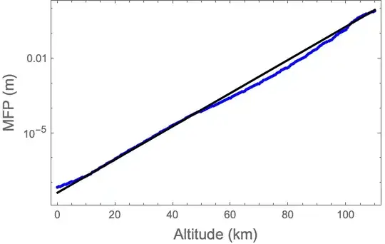
Show[ ListLogPlot[data, PlotStyle -> Blue], LogPlot[Exp[nlm2[x]], {x, 0, 110}, PlotStyle -> Black], Frame -> True, FrameLabel -> {Style["Altitude (km)", 14], Style["MFP (m)", 14]}]

enter image description here

EDIT: Alternatively, since

A*Exp[(x - B)*C] == Exp[Log[A]]*Exp[C*x - B*C] == 
  Exp[C*x - (B*C - Log[A])] // Simplify

(* True *)

The model has only two parameters. Use Exp[a*x + b]

To determine initial estimates for the NonlinearModelFit, use two widely separated data points

paramEst = 
 SolveValues[Exp[a*#[[1]] + b] == #[[2]] & /@ data[[{1, -1}]], {a, b}][[1]] //
   Quiet

(* {0.148094, -16.5286} *)

(nlm3 = NonlinearModelFit[data, Exp[a*x + b], Transpose[{{a, b}, paramEst}], x]) // Normal

(* E^(-17.0152 + 0.153491 x) *)

Show[ListLogPlot[data, PlotStyle -> Blue], LogPlot[nlm3[x], {x, 0, 110}, PlotStyle -> Black], Frame -> True, FrameLabel -> {Style["Altitude (km)", 14], Style["MFP (m)", 14]}]

enter image description here

Bob Hanlon
  • 157,611
  • 7
  • 77
  • 198
0

To long for a comment:

Mathematica v12.2 evaluates much better result as shown in your question. Try

<< StandardAtmosphere`
data = Table[{alt, MeanFreePath[alt Quantity[1, "Kilometers"]][[1]]}, {alt,0, 110, 0.5}];
nlm = NonlinearModelFit[data, A*Exp[(x - B)*C], {A, B, C}, x];
Show[ListLogPlot[data, PlotStyle -> Blue], 
LogPlot[nlm[x], {x, 0, 110}, PlotStyle -> Black], Frame -> True, 
FrameLabel -> {Style["Altitude (km)", 14], Style["MFP (m)", 14]}]

enter image description here

Ulrich Neumann
  • 53,729
  • 2
  • 23
  • 55
  • 1
    Thanks Ulrich! Unfortunately I just tried this verbatim in Mathematica 13.3 and I get the same result as in my post. – icebox207 Dec 02 '23 at 16:59