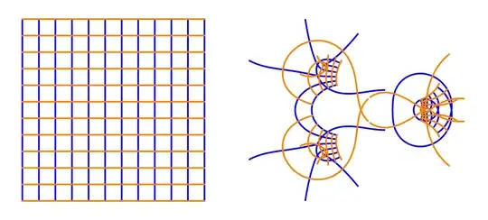
- We use
ParametricPlot to plot the mapping x+I*y -> ReIm[f[x+I*y]].
- We subdivide the original domain to
11x11 parts.
f[z_] := ProductLog[z^2] ProductLog[1/z];
plots = Block[{z = x + I*y},
    ParametricPlot[#, {x, -4, 4}, {y, -4, 4},
     Mesh -> {Subdivide[-4, 4, 11], Subdivide[-4, 4, 11]},
     MeshStyle -> {{Thick, Opacity[1], Blue}, {Thick, Opacity[1],
        Orange}}, PlotStyle -> None, Exclusions -> All,
     PlotPoints -> 100, MaxRecursion -> 2, Frame -> False,
     Axes -> False]] & /@ {ReIm[z], ReIm[f[z]]}
GraphicsRow[plots]
{f1, f2, f3, f4} = {BSplineFunction[{{.15, -4}, {.15, -.6}}],
  BSplineFunction[{{.15, 4}, {.15, .6}}],
  BSplineFunction[{{-2.8, 0.1}, {-.1, 0.1}, {-.3, .12}, {-.15, .2}}],
  BSplineFunction[{{-2.8, -0.1}, {-.1, -0.1}, {-.3, -.12}, {-.15, \
-.2}}]}; F = ReIm@*f@*({1, I} . # &);
plot1 = Block[{z = x + I*y},
   ParametricPlot[{f1@s, f2@s, f3@s, f4@s}, {s, 0, 1},
    PlotPoints -> 100, MaxRecursion -> 2, AspectRatio -> Automatic,
    PlotRange -> All, PlotStyle -> Directive@{Thick, Black}]];
plot2 = ParametricPlot[{F@*f1@s, F@*f2@s, F@*f3@s, F@*f4@s}, {s, 0,
    1}, PlotPoints -> 100, MaxRecursion -> 2,
   AspectRatio -> Automatic, PlotRange -> All, Exclusions -> None,
   PlotStyle -> Black];
GraphicsRow@{Show[plots[[1]], plot1], Show[plots[[2]], plot2]}


ComplexContourPlot[{Re[z], Im[z]}, {z, 10}]? Or perhaps would you rather make it more creative like e.g. here? – Artes Dec 22 '23 at 00:54ComplexContourPlot[{Re[z], Im[z]}, {z, 10}]. I'm not sure how the black lines are defined, though. – Goofy Dec 22 '23 at 01:50