Numerical solution to fractional PDE

Question

Following the idea here by @xzczd, I tried:

a = 1/10; t0 = 0; tend = 1/50; xL = 0; xR = 1;
{eq, ic, bc} = {CaputoD[y[t, x], {t, a}] == D[y[t, x], {x, 2}], 
y[t0, x] == Sin[Pi x], {y[t, xL] == 0, y[t, xR] == 0}};
nt = 15; range = Range[0, nt - 1];
coef[x_] = c[x] /@ range;
poly[x_][t_] = coef[x] . t^range;
domaint = {t0, tend};
CGLGrid[xl_, xr_, n_Integer /; n > 1] := 
1/2 (xl + xr + (xl - xr) Cos[(\[Pi] Range[0, n - 1])/(n - 1)])
gridt = CGLGrid[##, nt] & @@ domaint;
nx = 25; domainx = {xL, xR};
difforder = 2;
gridx = Array[# &, nx, domainx];
(*Definition of pdetoode isn't included in this post, please find it in the link above.*)
ptoofunc = pdetoode[y[t, x], t, gridx, difforder];
del = #[[2 ;; -2]] &;
{ode, odeic} = del /@ ptoofunc@{eq, ic};
odebc = ptoofunc@bc;
{approxode, approxic, approxbc} = {ode, odeic, odebc} /. 
y -> poly; // AbsoluteTiming
var = coef /@ gridx // Flatten;
sys = Flatten@{Table[approxode, {t, Rest@gridt}], 
Table[approxbc, {t, gridt}], approxic};
{barray, marray} = CoefficientArrays[sys, var]; 
csol = LinearSolve[marray, -N[barray, 32]];
Block[{c}, Evaluate@var = csol;
ParametricPlot3D[
Table[{t, x, poly[x][t]}, {x, gridx}] // Evaluate, {t, t0, tend}, 
PlotRange -> All, BoxRatios -> {1, 1, 0.4}]]
nsol = Block[{c}, Evaluate@var = csol;
ListInterpolation[Table[poly[x][t], {t, gridt}, {x, gridx}], {gridt, gridx}]];

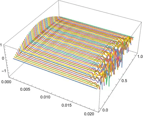
The plot gives

Let's compare with the analytical solution

sol3 = DSolve[{CaputoD[y[t, x], {t, a}] == D[y[t, x], {x, 2}], 
y[0, x] == Sin[Pi x], {y[t, 0] == 0, y[t, 1] == 0}}, y, {t, x}];
g[t_] := Integrate[Evaluate[y[t, x] /. sol3[[1]]]^2, {x, 0, 1}]

The plot gives Plot[{NIntegrate[nsol[t, x]^2, {x, 0, 1}], g[t]}, {t, t0, tend}]

My question is about the numerical issues in the above plot:

1. How to handle the oscillation near $0$?
2. How to get a smooth curve as in the analytical solution?

I tried to increase the number of points, e.g. nt=25 and nx=45, but the plot of lines become very different (oscillating near t=1/50) and second plot improves but still oscillating

Answer 1

There are several numerical methods to solve fractional PDE. In this case the best one could be implicit difference scheme described in this paper. The implementation is not so difficult compare to pdetode. We have

L = 1; tend = 1/50; dx = L/80; xgrid = Range[0, L, dx]; nn = 
 Length[xgrid];
M2 = NDSolve`FiniteDifferenceDerivative[Derivative[2], xgrid, 
    DifferenceOrder -> 2]@"DifferentiationMatrix";
wA = Table[wa[i][t], {i, nn}];
w2 = M2 . wA;
eq = Table[D[wA[[i]], t] == w2[[i]], {i, 2, nn - 1}];
bc = {wA[[1]] == 0, wA[[-1]] == 0};
ic = Table[
  wA[[i]] == Sin[Pi  xgrid[[i]]] /. t -> 0, {i, 2, nn - 1}]; icn = 
 Join[ic, bc /. t -> 0];
eqn = Join[eq, D[bc, t]]; var1 = D[wA, t];
sol[q_, nt1_] := 
  Module[{f, ff, vec, mat, cj, vij, dt, m, grid, nt, 
    eqq}, {vec, mat} = CoefficientArrays[eqn, var1];
   f = Inverse[mat // N] . (-vec);
   dt = tend/nt1; m = Length[f]; grid = Range[0, tend, dt]; 
   nt = Length[grid]; vij = Table[wA[[i]], {t, grid}, {i, m}];
   ff = Table[ f, {t, grid}];
   cj = Table[(j + 1)^(1 - q) - j^(1 - q), {j, nt}]; 
   eqAll = Flatten[
     Table[dt^(-q)/
         Gamma[2 - q] (vij[[n, i]] - vij[[n - 1, i]] + 
          Sum[(vij[[n - j + 1, i]] - vij[[n - j, i]]) cj[[j]], {j, 1, 
            n - 1}]) - ff[[n, i]], {n, 2, nt}, {i, m}]];
   varALL = Flatten[vij];
   so = FindRoot[
     Join[Table[eqAll[[i]] == 0, {i, Length[eqAll]}], icn], 
     Table[{varALL[[i]], .1}, {i, Length[varALL]}], 
     Method -> {"Newton", "StepControl" -> "TrustRegion"}, 
     MaxIterations -> 1000]; so];

Note, that solver sol[] is universal one. We can use it to solve nonlinear problems as well. Example of usage

sol01 = sol[1/10, 20];

Visualization

ListPointPlot3D[
 Table[{t, xgrid[[i]], wA[[i]] /. sol01}, {i, nn}, {t, 
    Range[0, tend, tend/20]}] // Evaluate, PlotRange -> All,AxesLabel -> {"t", "x", "y"}]

We can compare numerical solution with exact solution

y = Function[{t, x}, 
  MittagLefflerE[1/10, -\[Pi]^2 t^(1/10)] Sin[\[Pi] x]]
Table[Show[
  Plot[y[t, x], {x, 0, 1}, PlotStyle -> Blue, PlotRange -> All, 
   AxesLabel -> {"x", "y"}, PlotLabel -> N[t]], 
  ListLinePlot[Transpose[{xgrid, wA /. sol01}], 
   PlotStyle -> {Red, Dashed}]], {t, Range[0, tend, tend/20]}]

We see a large discrepancies on first two steps. But after that numerical solution comes to exact solution. Unfortunately this is common problem for all implicit schemas described in the paper sited. This scheme has an order $2-\alpha$ in $L_2$ norm. We can improve this code using higher order difference scheme from the paper cited

(*Caputo numerical derivative with order of accuracy 3-\[Alpha]*)
a[j_][q_] := (j + 1)^(1 - q) - j^(1 - q);
b[j_][q_] := ((j + 1)^(2 - q) - j^(2 - q))/(2 - 
      q) - ((j + 1)^(1 - q) + j^(1 - q))/2;
(*Fractional equations numerical solution*)       
sol12[q_, nt_] := 
  Module[{f, ff, vec, mat, c, vij, dt, m, grid, eqA}, {vec, mat} = 
    CoefficientArrays[eqn, var1];
   f = Inverse[mat // N] . (-vec);
   dt = tend/(nt - 1); m = Length[f]; grid = Range[0, tend, dt]; 
   vij = Table[wA[[i]], {t, grid}, {i, m}];
   ff = Table[f, {t, grid}]; eqA = Table[0, {nt - 1}, {m}];
   Do[Do[c[0] = If[n == 1, 1, a[0][q] + b[0][q]]; 
      If[n >= 2, 
       Do[c[j] = a[j][q] + b[j][q] - b[j - 1][q];, {j, 1, n - 2}]; 
       c[n - 1] = a[n - 1][q] - b[n - 2][q]]; 
      eqA[[n - 1, i]] = 
       dt^(-q)/Gamma[2 - q] (c[0] vij[[n, i]] - c[n - 1] vij[[1, i]] -
            Sum[(c[n - j - 1] - c[n - j]) vij[[j, i]], {j, 1, 
             n - 1}]) - ff[[n, i]];, {n, 2, nt}];, {i, m}];
   varALL = Flatten[vij]; eqAll = Flatten[eqA];
   {res, {evx}} = 
    Reap[FindRoot[
      Join[Table[eqAll[[i]] == 0, {i, Length[eqAll]}], icn], 
      Table[{varALL[[i]], .1}, {i, Length[varALL]}], 
      Method -> {"Newton", "StepControl" -> "TrustRegion"}, 
      MaxIterations -> 1000, EvaluationMonitor :> Sow[varALL]]]; 
   L2 = Table[
     Norm[evx[[k]][[1]] - evx[[k + 1]][[1]]], {k, 
      Length[evx] - 1}]; {res, evx, L2}];
sol012 = sol12[1/10, 21][[1]]; // AbsoluteTiming
Table[Show[
  Plot[y[t, x], {x, 0, 1}, PlotStyle -> Blue, PlotRange -> All, 
   AxesLabel -> {"x", "y"}, PlotLabel -> N[t]], 
  ListLinePlot[Transpose[{xgrid, wA /. sol012}], 
   PlotStyle -> {Red, Dashed}]], {t, Range[0, tend, tend/20]}]