How do I find the best fit?

Question

I am trying to solve following system of three differential equations

r = {
  -cab'[t] == k*cab[t] - kb*ca[t]*cb[t],
  ca'[t] == k*cab[t] - kb*ca[t]*cb[t],
  cb'[t] == k*cab[t] - kb*ca[t]*cb[t],
  cab[0] == 0.071176,
  ca[0] == 0.003697,
  cb[0] == 0.002845
};

and fit them to the following experimental data

cab = {0.071176, 0.05493, 0.04287, 0.03391, 0.02767, 0.02355, 
       0.02096,0.01825, 0.017029, 0.016582, 0.01421, 0.01432, 0.01431};
ca = {0.003697, 0.021051, 0.033007, 0.04154, 0.047609,0.052086, 0.05529, 
      0.057088, 0.05842, 0.05966, 0.06114, 0.06079,0.06153};
cb = {0.002845, 0.01949, 0.03078, 0.03714, 0.04476, 0.04939, 0.05214, 
      0.05327, 0.05526, 0.05573, 0.05859, 0.05774, 0.05868};
t = {0, 3600, 7200, 10800, 14400, 18000, 21600, 25200, 28800, 32400,82800, 86400, 90000};

I want to get the best k and kb values. Could you help me since I am novice in Mathematica. I would like a step-by-step tutorial on hoe to do it.

Answer 1

Rather than looking for a solution of the differential equations including the initial conditions, I'd postpone imposing them to when one does the fit. The solution will contain 3 constants to be determined based on the initial conditions :

{solca[t_], solcab[t_], solcb[t_]} = 
  DSolve[{-cab'[t] == k*cab[t] - kb*ca[t]*cb[t], 
            ca'[t] == k*cab[t] - kb*ca[t]*cb[t], 
            cb'[t] == k*cab[t] - kb*ca[t]*cb[t]}, 
    {cab[t], ca[t], cb[t]}, t][[1, All, 2]]

You might notice that the three solutions only differ by a constant (and a sign), which is obvious when looking at your system. Our model is a function which reproduces each solution to the system for index=1,2 or 3; we also need to rename the integration constants so we can manipulate them later.

f[index_, t_] = KroneckerDelta[index, 1] solca[t] + 
                KroneckerDelta[index, 2] solcab[t] + 
                KroneckerDelta[index, 3] solcb[t] /. {C[1] -> c1, C[2] -> c2, C[3] -> c3};

The next step would be to use FindFit to get the parameters k, kb; however they appear in 3 different functions and we want to have a common fit. I'll use a trick I learned here.

datacab = {0.071176, 0.05493, 0.04287, 0.03391, 0.02767, 0.02355, 0.02096, 0.01825, 0.017029, 0.016582, 0.01421, 0.01432, 0.01431};
dataca = {0.003697, 0.021051, 0.033007, 0.04154, 0.047609, 0.052086, 0.05529, 0.057088, 0.05842, 0.05966, 0.06114, 0.06079, 0.06153};
datacb = {0.002845, 0.01949, 0.03078, 0.03714, 0.04476, 0.04939, 0.05214, 0.05327, 0.05526, 0.05573, 0.05859, 0.05774, 0.05868};
datat = {0, 3600, 7200, 10800, 14400, 18000, 21600, 25200, 28800, 32400, 82800, 86400, 90000};

data = Join[Thread[List[1, datat, dataca]], 
            Thread[List[2, datat, datacab]], 
            Thread[List[3, datat, datacb]]]

Now data is in a suitable form to be taken as our experimental data for our model. We can also impose the initial conditions as part of the fitting.

solfit = 
FindFit[data, {f[index, t], f[2, 0] == 0.071176, f[1, 0] == 0.003697, f[3, 0] == 0.002845}, 
 {k, kb, c1, c2, c3}, {index, t}, Method -> NMinimize]
(* {k -> 0.298832, kb -> 3.07733, c1 -> 0.074873, c2 -> -0.00085201, c3 -> -1.95533} *)

Check :

f[1, 0] /. solfit // Chop
f[2, 0] /. solfit // Chop
f[3, 0] /. solfit // Chop
(* 0.003697
   0.071176
   0.00284499 *)

Finally we can put model and best fit together, do some manipulations to remove apparent imaginary parts and define our final solution ;

solution[index_, t_] = 
 Simplify[ComplexExpand[f[index, t] /. solfit, TargetFunctions -> {Re, Im}], 
  Assumptions -> {KroneckerDelta[__] \[Element] Reals}]

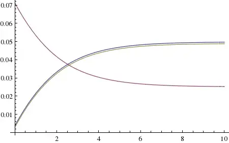
Plot[{solution[1, t], solution[2, t], solution[3, t]}, {t, 0, 10}]

Answer 2

I have modyfied my script. But now, the fitting is done taking into account only one set of date - datacab. Do you know how to change it so that minimization was done based on 3 sets of data (datacab, dataca, datacb)

datacab = {0.071176, 0.05493, 0.04287, 0.03391, 0.02767, 0.02355, 0.02096, 0.01825,
0.017029, 0.016582, 0.01421, 0.01432, 0.01431};
dataca = {0.003697, 0.021051, 0.033007, 0.04154, 0.047609, 0.052086, 0.05529,
0.057088, 0.05842, 0.05966, 0.06114, 0.06079, 0.06153};
datacb = {0.002845, 0.01949, 0.03078, 0.03714, 0.04476, 0.04939, 0.05214, 0.05327,
0.05526, 0.05573, 0.05859, 0.05774, 0.05868};
datat = {0, 3600, 7200, 10800, 14400, 18000, 21600, 25200, 28800, 32400, 82800,
86400, 90000};
ll = Length[datat];
dane = ListPlot[Table[{{datat[[i]], datacab[[i]]}, {datat[[i]], 
 dataca[[i]]}, {datat[[i]], datacb[[i]]}},{i, 1, ll}], PlotStyle -> PointSize[0.02]];
Clear[k1, k2];
kk1 = 0.00007;
kk2 = 0.000274;
Equation[k1_?NumberQ, k2__?NumberQ] = {-cab'[t] == k1*cab[t] - k2*ca[t]*cb[t], ca'[t] == k1*cab[t] - k2*ca[t]*cb[t], cb'[t] == k1*cab[t] - k2*ca[t]*cb[t], cab[0] == 0.071176,ca[0] == 0.003697, cb[0] == 0.002845};
Clear[chi2];
chi2[k1_?NumberQ, k2_?NumberQ] := (sol = 
cab /. NDSolve[Equation[k1, k2], {cab, ca, cb}, {t, 0, 90000}] // 
 First; (sol /@ datat) - datacab // #.# &);
Clear[k1, k2]
st = NMinimize[{chi2[k1, k2], k1 > 0, k2 > 0}, {k1, k2}]
k1 = st[[2, 1, 2]];
k2 = st[[2, 2, 2]];
eq = {-cab'[t] == k1*cab[t] - k2*ca[t]*cb[t], ca'[t] == k1*cab[t] - k2*ca[t]*cb[t], cb'[t] == k1*cab[t] - k2*ca[t]*cb[t], cab[0] == 0.071176, ca[0] == 0.003697, cb[0] == 0.002845};
sol = NDSolve[eq, {cab, ca, cb}, {t, 0, 90000}];
ff = Plot[Evaluate[{cab[t], ca[t], cb[t]} /. sol], {t, 0, 90000}, PlotStyle -> {Red, Thick}];
Show[ff, dane]