NDSolve FEM-Solver fails for simple PDE

Question

Trying to solve this pde (inspired by this question NeumannValue when differential equation does not use Laplacian )

pde = Derivative[2, 0][f][x, y] ==y^2*f[x, y] + NeumannValue[1, x == 1 ]
bc = DirichletCondition[f[x, y] == 1, x == 1]  ;
F = NDSolveValue[{pde, bc}, f, {x, 0, 1}, {y, 0, 1}] ;
Plot[{Derivative[1, 0][F][1, y] }, {y, 0, 1},GridLines -> {None, {1}}, PlotRange -> {0, 1},PlotLabel ->"NeumannValue[1,x\[Equal]1] isn't fullfilled!" ]

In contrast to that solution my "handmade Galerkin method" gives a smooth result, which fullfills the Neumann condition quite well

(If of interest here my code handmade Galerkin method )

I'm aware that NeumanValue in the first example is ignored because of DirichletCondition at the same boundary.

My question :

Is it possible to make FEM solution work for the case that Neumann and Dirichlet bcs are defined at the same place?

Thanks!

Answer 1

To verifier solution computed with Galerkin method we can use the Euler wavelets collocation method from my answer here. We add boundary conditions at y==0 and y==1 in a form of homogenous Neumann condition or in a form of pde. First version

UE[m_, t_] := EulerE[m, t];
psi[k_, n_, m_, t_] := 
  Piecewise[{{2^(k/2) UE[m, 2^k t - 2 n + 1], (n - 1)/2^(k - 1) <= t <
       n/2^(k - 1)}, {0, True}}];
PsiE[k_, M_, t_] := 
 Flatten[Table[psi[k, n, m, t], {n, 1, 2^(k - 1)}, {m, 0, M - 1}]]
k0 = 3; M0 = 4; With[{k = k0, M = M0}, 
 nn = Length[Flatten[Table[1, {n, 1, 2^(k - 1)}, {m, 0, M - 1}]]]];
dx = 1/(nn); xl = Table[l*dx, {l, 0, nn}]; zcol = 
 xcol = Table[(xl[[l - 1]] + xl[[l]])/2, {l, 2, nn + 1}]; Psijk = 
 With[{k = k0, M = M0}, PsiE[k, M, t1]]; Int1 = 
 With[{k = k0, M = M0}, Integrate[PsiE[k, M, t1], t1]];
Int2 = Integrate[Int1, t1];
Psi[y_] := Psijk /. t1 -> y; int1[y_] := Int1 /. t1 -> y;
int2[y_] := Int2 /. t1 -> y;
M = nn;
U1 = Array[a, {M, M}]; U2 = Array[b, {M, M}]; G1 = 
 Array[g1, {M}]; G2 = Array[g2, {M}]; G3 = Array[g3, {M}]; G4 = 
 Array[g4, {M}];
u1[x_, z_] := int2[x] . U1 . Psi[z] + x G1 . Psi[z] + G4 . Psi[z];
u2[x_, z_] := Psi[x] . U2 . int2[z] + z G2 . Psi[x] + G3 . Psi[x];
uz[x_, z_] := Psi[x] . U2 . int1[z] + G2 . Psi[x];
ux[x_, z_] := int1[x] . U1 . Psi[z] + G1 . Psi[z];
uxx[x_, z_] := Psi[x] . U1 . Psi[z];
uzz[x_, z_] := Psi[x] . U2 . Psi[z];
(Equations and solution)
eqn = Join[
  Flatten[Table[(uxx[xcol[[i]], zcol[[j]]] - 
      zcol[[j]]^2 u1[xcol[[i]], zcol[[j]]]), {i, M}, {j, M}]], 
  Flatten[Table[
    u1[xcol[[i]], zcol[[j]]] - u2[xcol[[i]], zcol[[j]]], {i, M}, {j, 
     M}]]]; bc = 
 Join[Flatten[Table[ux[1, zcol[[j]]] - 1 == 0, {j, M}]], 
  Flatten[Table[u1[1, zcol[[j]]] - 1 == 0, {j, 1, M}]], 
  Flatten[Table[uz[xcol[[j]], 0] == 0, {j, M}]], 
  Flatten[Table[uz[xcol[[j]], 1] == 0, {j, M}]]]; var = 
 Join[Flatten[U1], Flatten[U2], G1, G2, G3, G4];
eq = Join[Table[eqn[[i]] == 0, {i, Length[eqn]}], 
    bc];
{v, m} = CoefficientArrays[eq, var];
sol1 = LinearSolve[m // N, -v];
(Visualization)
rul = Table[var[[i]] -> sol1[[i]], {i, Length[var]}];
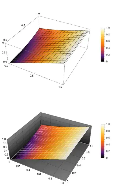
Plot3D[Evaluate[u1[x, y] /. rul], {x, 0, 1}, {y, 0, 1}, 
 PlotLegends -> Automatic, ColorFunction -> "SunsetColors", 
 PlotRange -> All, Exclusions -> None]
Plot3D[Evaluate[u2[x, y] /. rul], {x, 0, 1}, {y, 0, 1}, 
 PlotLegends -> Automatic, ColorFunction -> "SunsetColors", 
 PlotRange -> All, Exclusions -> None, PlotTheme -> "Marketing", 
 MeshStyle -> White]

In second version we use pde as follows

eq0 = Join[Table[uxx[xcol[[i]], 0] == 0, {i, M}], 
   Table[uxx[xcol[[i]], 1] - u1[xcol[[i]], 1] == 0, {i, M}]];
eq1 = eq = 
  Join[Table[eqn[[i]] == 0, {i, Length[eqn]}], Take[bc, 2 M], 
   eq0]; sol2 = CoefficientArrays[eq1, var]
sol = LeastSquares[sol2[[2]] // N, -sol2[[1]]] 

Solution sol is not differ from shown above sol1, which is already obvious.

Update 1. We can compare solution u1[x,y]/.rul and u1[x,y]/.rul1 with

sol3 = NDSolveValue[{Derivative[2, 0][f][x, y] == 
    y^2*f[x, y], {f[1, y] == 1, Derivative[1, 0][f][1, y] == 1}}, 
  f, {x, 0, 1}, {y, 0, 1}]

We have

{Plot[Table[Abs[sol3[x, y] - u1[x, y] /. rul1], {x, 0, 1, .1}] // 
   Evaluate, {y, 0, 1}, FrameLabel -> {"y", "\[Delta]f"}, 
  PlotLegends -> Automatic, Frame -> True, 
  PlotLabel -> "Absolute error for `pde` at y=0,1"], 
 Plot[Table[Abs[sol3[x, y] - u1[x, y] /. rul], {x, 0, 1, .1}] // 
   Evaluate, {y, 0, 1}, FrameLabel -> {"y", "\[Delta]f"}, 
  PlotLegends -> Automatic, Frame -> True, 
  PlotLabel -> "Absolute error for NeumannValue[0,y==0||y==1]"]}

Answer 2

This is not an answer but an extended comment. I think it would be good to simplify and speed up your code and make sure the FEM computations are correct. Following the FEM Programming tutorial we get this:

Needs["NDSolve`FEM`"]
pde = Derivative[2, 0][f][x, y] == 
   y^2*f[x, y] + NeumannValue[1, x == 1];
bc = DirichletCondition[f[x, y] == 1, x == 1];
F = data[{pde, bc}, f, {x, 0, 1}, {y, 0, 1}];

Using

NDSolveValue @@ F

gives what you had. This makes sure that we use the same input for NDSolveValus and for the system matrix extraction. Next we extract the system matrices:

{dPDE, dBC, vd, sd, md} = NDSolve`FEM`ProcessPDEEquations @@ F;
sm = dPDE["StiffnessMatrix"];
lv = dPDE["LoadVector"];

Next, we deploy the boundary conditions:

DeployBoundaryConditions[{lv, sm}, dBC];

Solve the linear equations:

result = LinearSolve[sm, lv];

And post process the solution:

NDSolve`SetSolutionDataComponent[sd, "DependentVariables", 
  Flatten[result]];
ProcessPDESolutions[md, sd]

Now, this solve the equation in exactly the same way like NDSolve would solve the PDE. What we can do next, is ignore the DirichletCondition. This will give a warning but we want to extract the load vector as if the DirichletCondition did not overwrite it:

F = data[{pde(*,bc*)}, f, {x, 0, 1}, {y, 0, 1}];
{dPDE, dBC, vd, sd, md} = NDSolve`FEM`ProcessPDEEquations @@ F;
smDummy = dPDE["StiffnessMatrix"];
lv = dPDE["LoadVector"];
DeployBoundaryConditions[{lv, smDummy}, dBC];
lv

Now, you have the load vector with the NeumannValue deployed. In your notebook you transform the PDE into an optimization problem and I have some difficulty to understand what you are doing there. If you could show this minimization approach based on the stiffness matrix and the NeumannValue, that would be useful, for me to understand how you want to solve this.

Now, let's do another experiment. Now we ignore the DirichletBoundary condition altogether:

pde = Inactive[Div][{{-1, 0}, {0, 0}} . 
      Inactive[Grad][f[x, y], {x, y}], {x, y}] - y^2*f[x, y] == 
   NeumannValue[1, x == 1];
(*bc=DirichletCondition[f[x,y]==1,x==1];*)
F = data[{pde(*,bc*)}, f, {x, y} \[Element] mesh];

Proceed as before, now we get an expected message:

{dPDE, dBC, vd, sd, md} = NDSolve`FEM`ProcessPDEEquations @@ F;
sm = dPDE["StiffnessMatrix"];
lv = dPDE["LoadVector"];

DeployBoundaryConditions[{lv, sm}, dBC];
result = LinearSolve[sm, lv];
NDSolve`SetSolutionDataComponent[sd, "DependentVariables", 
  Take[Flatten[result], md["DegreesOfFreedom"]]];
{ifun} = ProcessPDESolutions[md, sd];

Now, we look at the result in the same way the OP has done:

Plot[Evaluate[{Derivative[1, 0][ifun][1, y], 
   Derivative[1, 0][ifun][0, y]}], {y, 0, 1}]

Answer 3

modified

Extended comment to answer @user21.

Meanwhile I could DiscretizePDE too. Here my code

{xMin, xMax, yMin, yMax} = {0, 1, 0, 1};
Needs["NDSolve`FEM`"]

meshing

mesh = ToElementMesh[Rectangle[{xMin, yMin}, {xMax, yMax}], 
"MaxCellMeasure" -> 0.0001 , 
"MeshElementType" -> "TriangleElement", "MeshOrder" -> 1] ;
index = MeshCells[MeshRegion[mesh], 0][[All, 1]];
rand = mesh["BoundaryElements"][[All, 1]] // Flatten[#, 1] &;
indexR = Flatten[rand ] // DeleteDuplicates;
pi = mesh["Coordinates"]; (* alle Punkte )
fi = Table[f[i], {i, 1, Length[pi]}];  ( Unbekannte DOFs *)
reg1 = ImplicitRegion[0 <= y <= yMax && x == xMax, {x, y}]; (* Randx[Equal]xMax) 
rand1 = Select[rand ,RegionMember[reg1, pi[[ #[[1]]]]] &&RegionMember[reg1, pi[[ #[[2]]]]] &];( an diesem Rand gilt f[xMax,y][Equal]1*)
indexR1 = Flatten[rand1] // DeleteDuplicates;

discretization

vd = NDSolve`VariableData[{"DependentVariables","Space"} -> {{f}, {x, y}}];
sd = NDSolve`SolutionData[{"Space"} -> {mesh}];
cdata = InitializePDECoefficients[vd, sd, 
"DiffusionCoefficients" -> {{  {{-1, 0}, {0, 0}}}}, 
"ReactionCoefficients" -> {{-y^2} }];
bcdata = InitializeBoundaryConditions[vd,sd, {{NeumannValue[1, x == 1]}}   ] 
mdata = InitializePDEMethodData[vd, sd];
(Discretization)
dpde = DiscretizePDE[cdata, mdata, sd] ;
{load, stiffness, damping, mass} = dpde["All"];
dbc = DiscretizeBoundaryConditions[bcdata, mdata, sd];
DeployBoundaryConditions[{load, stiffness}, dbc];

solution

RB1 = Map[fi[[#]] == 1 &, indexR1];
mini = NMinimize[{(stiffness.fi - Flatten[load]) . (stiffness.fi-Flatten[load]), RB1}, fi];
solfun = ElementMeshInterpolation[{mesh}, fi /. mini[[2]]];
Plot3D[ solfun[x, y] , {x, y} [Element] mesh, AxesLabel -> {x, y} ,
PlotRange -> {{0, 1}, All}[[-1]], MeshFunctions -> (#3 &)]

Plot [ {Derivative[1, 0][solfun][1, y],Derivative[1, 0][solfun][0, y]} , {y, 0, 1}]

The result shows , the two Neumann-conditions and the DirichletCondition are fullfilled quite well.

It seems to be possible to get plausible results with Galerkin method, even if we take NeumannValue and Dirichletcondition at the same place of the boundary!

addendum

With the last example (@user21 's extended comment) the minimization problem with matrices smdummy and lv follows after introducing the dirichletcondition

RB1 = Map[fi[[#]] == 1 &, indexR1];(* all meshpoints `x==1`*)
mini = NMinimize[{(smdummy.fi + Flatten[lv]) . (smdummy.fi+    Flatten[lv]), RB1}, fi];