Curve fitting with Mathematica

Question

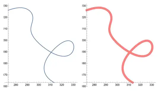
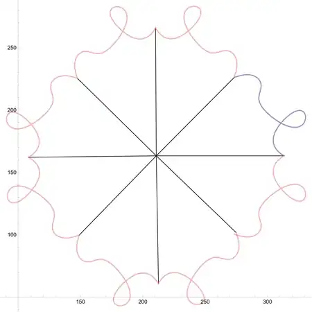
I am trying to find de parametric equations of this curve (the curve in that sector of circle):

What I've tried:

data = {{2.75, 2.7}, {3.1, 2.84}, {3.45, 2.97}, {3.76, 2.82}, {3.9, 2.45}, {3.72, 2.21}, {3.33, 2.13}, {3.36, 1.87}, {3.65, 1.63}, {3.93, 1.39}, {4.22, 1.15}, {4.55, 0.97}, {4.89, 0.8}, {5.25, 0.7}, {5.41, 1}, {5.4, 1.37}, {5.35, 1.74}, {5.11, 1.96}, {4.8, 1.74}, {4.51, 1.5}, {4.28, 1.21}, {4.06, 0.91}, {3.89, 0.57}, {4.11, 0.27}, {4.45, 0.11}, {2.75, 2.7}, {2.93, 2.79}, {3.18, 2.87}, {3.39, 2.95}, {3.63, 2.96}, {3.78, 2.78}, {3.88, 2.53}, {3.89, 2.27}, {3.63, 2.2}, {3.42, 2.15}, {3.23, 2.08}, {3.34, 1.9}, {3.52, 1.72}, {3.73, 1.58}, {3.91, 1.41}, {4.09, 1.29}, {4.25, 1.12}, {4.49, 1}, {4.74, 0.86}, {4.95, 0.78}, {5.18, 0.69}, {5.34, 0.73}, {5.39, 0.93}, {5.43, 1.11}, {5.41, 1.32}, {5.39, 1.55}, {5.34, 1.77}, {5.24, 1.97}, {5.07, 1.94}, {4.88, 1.81}, {4.71, 1.66}, {4.53, 1.52}, {4.38, 1.37}, {4.24, 1.15}, {4.07, 0.93}, {3.95, 0.75}, {3.89, 0.55}, {4, 0.36}, {4.2, 0.22}, {4.45, 0.11}}

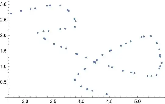
And this is what I've got:

Now I've tried to do some Bezier interpolation:

f = SplineFit[data, Bezier]
ParametricPlot[f[x], {x, 0, 62}]

And this is what I've got:

This seems to be quite ok. But I don't know how to extract parametric equations from here. Any idea? Thanks!

Welcome to the community. I'm not sure what version you're using but executing your code on version 14, gives a different output. Regardless of that quoting documentation "A Bézier curve can be constructed from the sum of the Bernstein polynomials:" 7th example under the "Properties & Relations" section. — Ben Izd, Mar 03 '24 at 18:18
@BenIzd i'm executing this code on version 14 too. But from that documentation I don't understand how I can view the parametric equations. — MathLearner, Mar 03 '24 at 18:28
Maybe your data is different. One could use PiecewiseExpand@ Module[{n = Length[data] - 1}, Sum[data[[i + 1]] BernsteinBasis[n, i, x], {i, 0, n}] ] to get the equations. — Ben Izd, Mar 03 '24 at 18:43

cvgmt · Accepted Answer · 2024-03-04T14:23:31.343

Your data have some duplicate points. We can use Mathematica to import the image and right click to Get Coordinates then use Ctrl + c to get the points.

img = Import["https://i.stack.imgur.com/MKUMm.png"]

SplineFit is an old package, now we can use BezierFunction[data] to replace SplineFit[data, Bezier], and it is also the same as bezierFunction which we directly define as below. (cf. https://mathematica.stackexchange.com/a/251536/72111)

bezierFunction[pts_][t_] := 
  Module[{n = Length@pts}, 
   Sum[Binomial[n - 1, i - 1] t^(i - 1) (1 - t)^(n - 1 - (i - 1))*
     pts[[i]], {i, 1, n}]];

Clear["Global`*"];
data = {{313.2857142857143, 
    163.29310825892853`}, {307.92857142857144`, 
    166.50739397321425`}, {302.92857142857144`, 
    170.4359654017857}, {299.7142857142857, 
    176.50739397321425`}, {303.2857142857143, 
    184.00739397321425`}, {307.2142857142857, 
    186.8645368303571}, {310.42857142857144`, 
    191.50739397321425`}, {316.14285714285717`, 
    196.50739397321425`}, {320.7857142857143, 
    201.50739397321425`}, {325.07142857142856`, 
    204.3645368303571}, {329.3571428571429, 
    207.9359654017857}, {332.57142857142856`, 
    205.07882254464286`}, {334., 
    201.50739397321425`}, {334.7142857142857, 
    195.4359654017857}, {334.7142857142857, 
    189.3645368303571}, {334.7142857142857, 
    184.00739397321425`}, {331.5, 
    178.29310825892853`}, {325.07142857142856`, 
    178.29310825892853`}, {320.42857142857144`, 
    181.15025111607142`}, {315.07142857142856`, 
    184.3645368303571}, {310.42857142857144`, 
    186.50739397321425`}, {305.7857142857142, 
    190.79310825892856`}, {301.14285714285705`, 
    195.07882254464283`}, {296.8571428571428, 
    198.29310825892858`}, {291.14285714285717`, 
    202.9359654017857}, {287.2142857142857, 
    206.50739397321425`}, {285.4285714285714, 
    209.36453683035717`}, {290.07142857142856`, 
    212.9359654017857}, {292.9285714285714, 
    212.57882254464283`}, {297.57142857142856`, 
    214.00739397321425`}, {300.7857142857143, 
    216.8645368303571}, {298.6428571428571, 
    223.29310825892856`}, {295.7857142857143, 
    229.0073939732143}, {291.14285714285717`, 
    230.07882254464283`}, {284.71428571428567`, 
    230.4359654017857}, {280.4285714285714, 
    227.9359654017857}, {276.1428571428571, 
    227.22167968750003`}, {273.2857142857143, 226.15025111607142`}};
n = Length@data;
center = {210.78571428571428`, 163.29310825892853`};
Needs["Splines`"];
f = SplineFit[data, Bezier];
plot1 = ParametricPlot[f[x], {x, 0, Length@data}];
(*bezierFunction[pts_][t_]:=Module[{n=Length@pts},Sum[BernsteinBasis[\
n-1,i-1,t]*pts[[i]],{i,1,n}]];*)
bezierFunction[pts_][t_] := 
  Module[{n = Length@pts}, 
   Sum[Binomial[n - 1, i - 1]   t^(i - 1)   (1 - t)^(n - 1 - (i - 1))*
     pts[[i]], {i, 1, n}]];
expr = bezierFunction[data][t];
plot2 := 
  ParametricPlot[expr, {t, 0, 1}, 
   PlotStyle -> 
    Directive@{RandomColor[], Opacity[.5], AbsoluteThickness[2]}];
{plot1, plot2}
expr

For the full graphics.

p1 = data[[1]];
p2 = data[[-1]]; 
pts = 
 SequenceFoldList[
  ReflectionTransform[Cross[#2 - center], center]@#1 &, {p1, p2}, 
  Range[5], 2];
Graphics[{Line[{center, #}] & /@ pts, First@plot2, 
  GeometricTransformation[First@plot2, 
   FoldList[RightComposition, 
    Table[ReflectionTransform[Cross[pts[[i]] - center], center], {i, 
      Range[Length@pts - 1]}]]]}, Axes -> True]

Thank you! This is perfect! – MathLearner Mar 04 '24 at 21:17 — MathLearner, Mar 04 '24 at 21:17

Curve fitting with Mathematica

1 Answers1