FindRoot changes results from ParametricNDSolve

Question

I solve numerically an equation, and I get the expected behaviour like the following graph

But if I use FindRoot to get the roots before plotting, the plot of my solution changes drastically:

This is the code I am using

σs = .18;
{α2, mc} = {-0.1185, 1.27`};
bc[r_] = AiryAi[(-e mc + mc r σs)/(mc σs)^(2/3)];
inf = 20;
usol = ParametricNDSolve[{-(1/mc)*D[u[r], {r, 2}] + (α2/r + σs*r)*u[r] == e*u[r], 
    u[inf] == bc[inf], u'[inf] == bc'[inf]}, u, {r, 10^-10, inf}, e][[1, 2]]
Plot[usol[p][10^-10], {p, 0, 2.5}]
FindRoot[usol[p][10^-10], {p, 2}]
Plot[usol[p][10^-10], {p, 0, 2.5}]

Welcome to Mathematica StackExchange! I can confirm this weird (and in my opinion buggy) behaviour in v12.3, v13.0 and v14.0. The reason for this is that ParametricNDSolve uses caching, and FindRoot seems to be evaluating the function differently, and repopulating the cache with "wrong"/less accurate values. You can do ParametricNDSolve[..., Method -> {"ParametricCaching" -> None}], but I believe this should be fixed by developers, nevertheless. — Domen, Mar 28 '24 at 13:12
Thanks for the explanation, I'm using Mathematica v14.0 but even using the ParametricNDSolve[..., Method -> {"ParametricCaching" -> None}] remains buggy, but at least now I know why, I hope it will be fixed in the next versions. — William Santos, Mar 28 '24 at 17:25
Sorry, you are right, you have to also turn off caching the derivative Method -> {"ParametricCaching" -> None, "ParametricSensitivity" -> None}. This should work now :) — Domen, Mar 28 '24 at 17:33
This absolutely shouldn't happen and should be reported as a bug. — march, Mar 28 '24 at 18:36

Michael E2 · Accepted Answer · 2024-03-31T13:31:04.147

I believe the culprit is differentiating usol[p][10^-10]. It looks like numerical ill-conditioning. However, I don't think differentiation should affect the numerics of the undifferentiated solution. So report it to WRI.

\[Sigma]s = .18;
{\[Alpha]2, mc} = {-0.1185, 1.27`};
bc[r_] = AiryAi[(-e  mc + mc  r  \[Sigma]s)/(mc  \[Sigma]s)^(2/3)];
inf = 20;
usol = ParametricNDSolveValue[{-(1/mc)*
       D[u[r], {r, 2}] + (\[Alpha]2/r + \[Sigma]s*r)*u[r] == e*u[r], 
    u[inf] == bc[inf], u'[inf] == bc'[inf]}, u, {r, 10^-10, inf}, e];
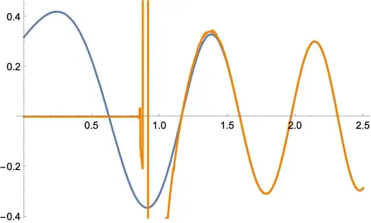
p1 = Plot[usol[p][10^-10], {p, 0, 2.5}];
D[usol[p][10^-10], {p}] /. p -> 0;  (*** <--- N.B.--- ***)
p2 = Plot[usol[p][10^-10], {p, 0, 2.5}, PlotStyle -> Orange];
Show[p1, p2]

Fix one:

Don't allow differentiation (with respect to e) in ParametricNDSolve[]:

usol = ParametricNDSolveValue[{-(1/mc)*
      D[u[r], {r, 2}] + (\[Alpha]2/r + \[Sigma]s*r)*u[r] == e*u[r], 
   u[inf] == bc[inf], u'[inf] == bc'[inf]}, u, {r, 10^-10, inf}, e, 
  Method -> {"ParametricSensitivity" -> None}]

Fix two:

Prevent differentiation (with respect to e) in FindRoot:

obj[p_?NumericQ] := usol[p][10^-10];
FindRoot[obj[p], {p, 2}]

Fix three:

Avoid differentiation (with respect to e) in FindRoot by using the secant method:

FindRoot[usol[p][10^-10], {p, 2, 2.1}]

Fix four:

High precision integration (lower truncation error):

\[Sigma]s = .18;
{\[Alpha]2, mc} = {-0.1185, 1.27`};
bc[r_] = AiryAi[(-e  mc + mc  r  \[Sigma]s)/(mc  \[Sigma]s)^(2/3)];
inf = 20;
usol = ParametricNDSolveValue[{-(1/mc)*
       D[u[r], {r, 2}] + (\[Alpha]2/r + \[Sigma]s*r)*u[r] == e*u[r], 
    u[inf] == bc[inf], u'[inf] == bc'[inf]}, u, {r, 10^-10, inf}, e, 
   PrecisionGoal -> 12, AccuracyGoal -> 15];
p1 = Plot[usol[p][10^-10], {p, 0, 2.5}];
D[usol[p][10^-10], {p}] /. p -> 0;
p2 = Plot[usol[p][10^-10], {p, 0, 2.5}, PlotStyle -> Orange];
Show[p1, p2]

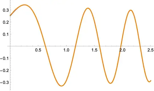
Note slight difference in plots for 0 < p < 0.1.

Fix five:

High precision numerics (lower round-off error):

\[Sigma]s = .18`32;
{\[Alpha]2, mc} = {-0.1185`32, 1.27`32};
bc[r_] = AiryAi[(-e  mc + mc  r  \[Sigma]s)/(mc  \[Sigma]s)^(2/3)];
inf = 20;
usol = ParametricNDSolveValue[{-(1/mc)*
       D[u[r], {r, 2}] + (\[Alpha]2/r + \[Sigma]s*r)*u[r] == e*u[r], 
    u[inf] == bc[inf], u'[inf] == bc'[inf]}, u, {r, 10^-10, inf}, e, 
   WorkingPrecision -> 32, PrecisionGoal -> 6];
p1 = Plot[usol[p][10^-10], {p, 0, 2.532}, PlotStyle -&gt; AbsoluteThickness[4], WorkingPrecision -&gt; 32]; D[usol[p][10^-10], {p}] /. p -&gt; 0; p2 = Plot[usol[p][10^-10], {p, 0, 2.532}, PlotStyle -> Orange, 
   WorkingPrecision -> 32];
Show[p1, p2]

azerbajdzan · Answer 2 · 2024-03-28T19:42:30.827

The only difference usol := instead of usol =.

σs = .18;
{α2, mc} = {-0.1185, 1.27`};
bc[r_] = AiryAi[(-e mc + mc r σs)/(mc σs)^(2/3)];
inf = 20;
usol := ParametricNDSolve[{-(1/mc)*D[u[r], {r, 2}] + (α2/r + σs*r)*u[r] == e*u[r], 
    u[inf] == bc[inf], u'[inf] == bc'[inf]}, u, {r, 10^-10, inf}, e][[1, 2]]
Plot[usol[p][10^-10], {p, 0, 2.5}]
FindRoot[usol[p][10^-10], {p, 2}]
Plot[usol[p][10^-10], {p, 0, 2.5}]

Decide on your preference which definition you use, here are timings for original version with =, @Domen's version with = and Method and last version with :=.

Clear[usol1, usol2, usol3]
σs = .18;
{α2, mc} = {-0.1185, 1.27`};
bc[r_] = AiryAi[(-e mc + mc r σs)/(mc σs)^(2/3)];
inf = 20;
usol1 = ParametricNDSolve[{-(1/mc)D[u[r], {r, 2}] + (α2/r + σsr)u[r] == eu[r], 
    u[inf] == bc[inf], u'[inf] == bc'[inf]}, u, {r, 10^-10, inf}, e][[1, 2]]
usol2 = ParametricNDSolve[{-(1/mc)D[u[r], {r, 2}] + (α2/r + σsr)u[r] == eu[r], 
    u[inf] == bc[inf], u'[inf] == bc'[inf]}, u, {r, 10^-10, inf}, e, Method->{"ParametricCaching"->None,"ParametricSensitivity"->None}][[1, 2]]
usol3 := ParametricNDSolve[{-(1/mc)D[u[r], {r, 2}] + (α2/r + σsr)u[r] == eu[r], 
    u[inf] == bc[inf], u'[inf] == bc'[inf]}, u, {r, 10^-10, inf}, e][[1, 2]]
Print["usol="]
Table[usol1[q][10^-10], {q, 0, 2.5, 0.001}]; // Timing
Table[usol1[q][10^-10], {q, 0, 2.5, 0.001}]; // AbsoluteTiming
Print["usol= with method parameters"]
Table[usol2[q][10^-10], {q, 0, 2.5, 0.001}]; // Timing
Table[usol2[q][10^-10], {q, 0, 2.5, 0.001}]; // AbsoluteTiming
Print["usol:="]
Table[usol3[q][10^-10], {q, 0, 2.5, 0.001}]; // Timing
Table[usol3[q][10^-10], {q, 0, 2.5, 0.001}]; // AbsoluteTiming

This undermines the core idea of ParametricNDSolve, namely that you don't have to reevaluate NDSolve for every value of parameter. — Domen, Mar 28 '24 at 18:57
But turning off cashing like you suggest contradicts your assertion. — azerbajdzan, Mar 28 '24 at 19:15

FindRoot changes results from ParametricNDSolve

2 Answers2