How to plot the contour of the radius part of a complex function

Question

Suppose we have a complex function $f(x,y)$, in which x and y are real variables. In theory we can write the function into the polar form

$$ f(x,y)=r(x,y)e^{i\theta(xy)} $$

where $r(x,y)$ and $\theta(x,y)$ are real functions. For some complicated function, it may very difficult to see what $r(x,y)$ and $\theta(x,y)$ are. So my question is if given a the function $f(x,y)$, is it possible to plot the contour of the function $r(x,y)$:

$$r(x,y)=0$$

?

For example,

f[x_, y_] := (Cos[x] + Cos[y]) Exp[I x y]

how can I reproduce the contour of (Cos[x] + Cos[y])==0 only using $f[x,y]$?

Grid@{{ContourPlot[Re@f[x, y] == 0, {x, 0, 4 Pi}, {y, 0, 4 Pi}, 
    ImageSize -> 300],
   ContourPlot[Im@f[x, y] == 0, {x, 0, 4 Pi}, {y, 0, 4 Pi}, 
    ImageSize -> 300]}, {
   ContourPlot[(Cos[x] + Cos[y]) == 0, {x, 0, 4 Pi}, {y, 0, 4 Pi}, 
    ImageSize -> 300],
   ContourPlot[Abs[f[x, y]] == 0, {x, 0, 4 Pi}, {y, 0, 4 Pi}, 
    ImageSize -> 300]}}

Here is more complicated function just for check

f[a_, a0_, k_, K0_]:=E^(I a0 K0) (2 a - I k) LegendreP[2, (I k)/a, -Tanh[(a a0)/2]] (E^(I a0 K0)LegendreQ[1, (I k)/a, -Tanh[(a a0)/2]] - LegendreQ[1, (I k)/a, Tanh[(a a0)/2]]) - (2 a - I k) LegendreP[2, (I k)/a, Tanh[(a a0)/2]] (E^(I a0 K0) LegendreQ[1, (I k)/a, -Tanh[(a a0)/2]] - LegendreQ[1, (I k)/a, Tanh[(a a0)/2]]) + E^(I a0 K0)LegendreP[1, (I k)/a, -Tanh[(a a0)/2]] (I E^(I a0 K0)k LegendreQ[2, (I k)/a, -Tanh[(a a0)/2]] + (2 a - I k) LegendreQ[2, (I k)/a, Tanh[(a a0)/2]]) + LegendreP[1, (I k)/a, Tanh[(a a0)/2]] (E^(I a0 K0) (2 a - I k) LegendreQ[2, (I k)/a, -Tanh[(a a0)/2]] + I k LegendreQ[2, (I k)/a, Tanh[(a a0)/2]] + 4 a E^(I a0 K0)LegendreQ[1, (I k)/a, -Tanh[(a a0)/2]] Tanh[(a a0)/2]) - 2 a (LegendreP[1, (I k)/a, Tanh[(a a0)/2]] LegendreQ[2, (I k)/a, Tanh[(a a0)/2]] + E^(I a0 K0)LegendreP[1, (I k)/a, -Tanh[(a a0)/2]] (E^(I a0 K0)LegendreQ[2, (I k)/a, -Tanh[(a a0)/2]] + 2 LegendreQ[1, (I k)/a, Tanh[(a a0)/2]] Tanh[(a a0)/2]))

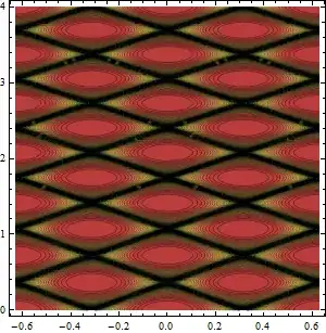
With[{a0 = 10., a = 1.4},
 Row@{ContourPlot[
    Re[f[a, a0, k, K0]] == 0, {K0, -2 \[Pi]/a0, 2 \[Pi]/a0}, {k, 0, 
     4}, ImageSize -> 400, PlotLabel -> "Re"],
   ContourPlot[
    Im[f[a, a0, k, K0]] == 0, {K0, -2 \[Pi]/a0, 2 \[Pi]/a0}, {k, 0, 
     4}, ImageSize -> 400, PlotLabel -> "Im"]}]

and I expect to get something like this

Note that this question is related to my another question here, where I tried to plot the contour of

$$ |f(x,y)|=|r(x,y)|=0 $$

but it turned out that plot the zero contour of a non-negative function is hard, since ContourPlot seems to be based on the Intermediate Value Theorem. Jens gives a manual approach in that question, but my future functions would be complicated Legendre and Hypergeometric functions, which would be a pain to manually deal with them by hand. So here I'm asking for maybe some alternative approaches to plot $r(x,y)=0$, if there are any.

Answer 1

Plotting the zero contour of a non-negative function is not hard. You do not need manual approaches. You just need to exaggerate the set that you need.

For your last example, I would use

With[{a0 = 10., a = 1.4}, 
  ContourPlot[Log[Abs[f[a, a0, k, K0]]], {K0, -2 \[Pi]/a0, 2 \[Pi]/a0}, {k, 0, 4},
   ImageSize -> 300, ColorFunction -> "DarkRainbow", 
   ClippingStyle -> Black, Contours -> 40]]