Jumps in NDSolve results

Question

I need to compute using NDSolve routine, some function $F(x)$, having two possible values $F_1(x)$ and $F_2(x)$ depending on whether the argument exceeds some critical value $x>x_c$. The problem is that NDSolve routine return "jumping results" for the region $x>x_c$.

As an example of a problem assume following system (some simple forced pendulum with nonlinear frequncy shift, so-called "fold over" effect):

w00 = 7000;
G0 = 50;
Q = 14000;
hU = 0.6*G0;
w0 = w00 - x;

(* example NDSolve call with sample value for x -- see below for actual usage *)
Block[{x = 8000},
 NDSolve[
  {A'[t] + G0*A[t] + I*(w0+Q*Abs[A[t]]^2)*A[t] == I*hU, A[0] == 10^-6}, 
  A[t], {t, 0, tmax},
  MaxSteps -> Infinity, AccuracyGoal -> 50, MaxStepSize -> 0.01
  ];
 ]

I am interested in $|A(t)|^2$ dynamics depending on the parameter x. Here $G0,Q,hU$ are some constants

Exact solution:

exact = ContourPlot[
  A == (hU^2/((G0)^2 + (w0 + Q*A)^2)),
  {t, 6000, 9000}, {A, 0, 0.2},
  PlotPoints -> 40, ContourStyle -> {Dashed, Thick},
  PlotRange -> All
]

Numerical solution:

Calc[x_] := Module[{
   w0 = 7000, G0 = 50, Q = 14000, At = 10^-6, tmax = 4,
   hU, w00, G1
  },

  hU = 0.6*G0;
  w00 = w0 - x + Q*Abs[A0[t]]^2;
  G1 = 1.0 G0;

  s2 = NDSolve[{
    A0'[t] + G0*A0[t] + I*w00*A0[t] == I*hU,
    A0[0] == 0.7 + 0.5 I
   }, A0[t], {t, 0, tmax}, 
   MaxSteps -> Infinity, AccuracyGoal -> 50, MaxStepSize -> 0.01
  ];

  {Abs[A0[t] /. s2 /. t -> tmax][[1]]}
]
Dynamic[z]
For[h1 = {}; z = 9000, z > 6000, z = z - 50,
 AppendTo[h1, {z, First@Calc[z]^2}];
]
numerical = ListPlot[h1, PlotRange -> All, Joined -> True, PlotStyle -> Thick]

Comparing both:

Show[exact, numerical]

Comparing NDSolve and exact solutions

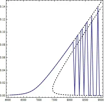
Solid line – NDSolve solution, dashed line - exact solution

The result and number of jumps greatly depends on initial conditions:

A[0] == 0.7 + 0.5*I

enter image description here

A[0] == 10^-6

enter image description here

The problem is I want to divide the two "branches" of the function $F_1$ and $F_2$ and plot them independently. How can I do this using NDSolve and force it to go along the chosen branch and not "jump?"?

To closers: yes, this is an old, unanswered question. But (a) it is upvoted, (b) OP has been seen only 2 months ago, and (c) I cannot agree that it is at all unclear. Potentially it is too localized, but I'm not sure about that. I appreciate the help but this is not quite what I had in mind by closing old questions. I think the best thing to do is to bounty it--please leave a comment if you think it should still be closed. — Oleksandr R., Sep 29 '15 at 21:27
I just evaluated the code and I ended up with lots of warnings, maybe it needs some cleaning up. — Raymond Ghaffarian Shirazi, Sep 29 '15 at 22:04
@RaymondGhaffarianShirazi thanks. I fixed the errors so that the OP's observations are reproducible now. — Oleksandr R., Sep 30 '15 at 00:24
Thanks, I give it look, I suspect I faced a similar challenge and those sloped vertical lines where produced by plot command actually. — Raymond Ghaffarian Shirazi, Sep 30 '15 at 00:48
@OleksandrR. Judging from the definition of Calc, I think the 5th line of code in the first code block, w0 = w00 - t, was meant to be w0 = w00 - x as originally written; I think what's missing is an example value for x. But that NDSolve in the first code block is superfluous. I will update the edit... — Michael E2, Sep 30 '15 at 10:15
@MichaelE2 thanks, I think you are right. To be honest, I wasn't sure if there was any benefit to having that listed there as well as later on. I didn't delete it only because apparently OP thought it was relevant. — Oleksandr R., Sep 30 '15 at 14:45

score 10 · Answer 1 · edited Apr 13 '17 at 12:55

(Update: I forgot to copy some of the code)

For values of z = x beyond the critical value (just below z == 7500), there are three real equilibria, two stable spirals and one (unstable) saddle.

eq[x_] := Module[{q = x},
   w0 = 7000;
   G0 = 50;
   Q = 14000;
   hU = 0.6*G0;
   w00 = w0 - q + Q*Abs[A0[t]]^2;
   At = 10^-6;
   G1 = 1.0 G0;
   tmax = 4;
   e1 = D[A0[t], t] + G0*A0[t] + I*w00*A0[t] == I*hU];

realeq[x_] := (* the real and imaginary parts in terms of A0[t] = u[t] + I v[t] *)
 ComplexExpand@
   Through[{Re, Im}[Subtract @@ eq[x] /. {A0 -> (u[#] + I v[#] &)}]] == {0, 0}

equil = NSolve[realeq[7575] /. {u'[t] -> 0, v'[t] -> 0}, {u[t], v[t]}, Reals]
(*
{{u[t] -> -0.163309,  v[t] -> 0.0483454},
 {u[t] ->  0.207442,  v[t] -> 0.0832793},
 {u[t] -> -0.0560372, v[t] -> 0.00528008}}
*)

Stability:

Det@D[First@realeq[7575] /. {u'[t] -> 0, v'[t] -> 0}, {{u[t], v[t]}}] /. equil
(*  {-106153., 192263., 237015.}  *)

StreamPlot[
 ComplexExpand@
  Through[{Re, Im}[
    A0'[t] /. First@Solve[eq[7575], A0'[t]] /. {A0[t] -> u + I v}]],
 {u, -0.3, 0.3}, {v, -0.3, 0.3}, 
 Epilog -> {PointSize[Medium], Green, Point[{u[t], v[t]} /. equil]},
 StreamPoints -> Fine]

Fig. 1. Phase plot with separatrices showing the basins of attraction.

As z changes, the basins of attraction for each spiral point change, and as they move, the initial conditions changes which basin it lies in.

Calc[x_] := Module[{q = x},
   w0 = 7000;
   G0 = 50;
   Q = 14000;
   hU = 0.6*G0;
   w00 = w0 - q + Q*Abs[A0[t]]^2;
   At = 10^-6;
   G1 = 1.0 G0;
   tmax = 4;
   e1 = D[A0[t], t] + G0*A0[t] + I*w00*A0[t] == I*hU;
   s2 = NDSolve[{e1, A0[0] == (0.7 + 0.5 I) + 0*10^-6}, {A0}, {t, 0, 
      tmax}, MaxSteps -> Infinity, AccuracyGoal -> 50, 
     MaxStepSize -> 0.01];
   {Evaluate[Abs[A0[t] /. s2 /. t -> tmax]][[1]]}];

movie = Table[Calc[z];
   ParametricPlot[Through[{Re, Im}[A0[t] /. s2]], {t, 0, 4}, 
    Epilog -> {PointSize[Medium], Red, 
      Point[Through[{Re, Im}[A0[4] /. First@s2]]], Green, 
      Point[{u[t], v[t]} /. 
        NSolve[ComplexExpand@
           Through[{Re, Im}[
             Subtract @@ e1 /. {A0[t] -> u[t] + I v[t], A0'[t] -> 0}]] == {0, 0},
         {u[t], v[t]}, Reals]]},
    PlotRange -> 1, MaxRecursion -> 15,
    PlotLabel -> HoldForm["z"] == z],
   {z, 7550, 7650}];

To get a result like the one the OP wants, one would need to adjust the initial condition as a function of z. But if, as it seems, the OP just wants to get a function representing the curve in the contour plot, one could use a different method, such as the ones I used here:

Jumps in NDSolve results

1 Answers1

Linked