I am trying to get plot for the band structure for graphene.
d = 10; (*Plot range*)
coupling := {{0, 2 Cos[Sqrt[3]*(#1)/2]*Cos[#2/2] + Cos[#2] +
I (2 Cos[Sqrt[3]*(#1)/2]*Sin[#2/2] - Sin[#2])},
{Conjugate[ 2 Cos[Sqrt[3]*(#1)/2]*Cos[#2/2] + Cos[#2] +
   I (2 Cos[Sqrt[3]*(#1)/2]*Sin[#2/2] - Sin[#2])], 0}} &;
Plot3D[Eigenvalues[coupling[kx, ky]][[1]], {kx, -d, d}, {ky, -d, d}] (*Discontinuous*)
Plot3D[(Eigenvalues[coupling[kx, ky]][[1]])^2, {kx, -d, d}, {ky, -d, d}] (*Continuous*)
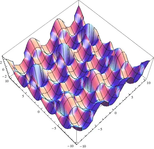
I am not able to understand why the surface in the first plot is coming out discontinuous; i.e., it has some gaps in the surface plot, whereas there are no gaps in the second plot, which simply plots the square of the function shown in the first plot.
There is no physics that explains the gaps. Also, the effect is not periodic/predictable. By that I mean that on changing d, I am getting very different patterns of gaps all over the place.
Is there some problem with my code or is 3D plot working incorrectly? How do I get rid of this error?
Edit
I am NOT talking about the spike at (0,0). I am attaching a picture of my plot for clarity. I am talking about the "ribbons" missing from the surface.

There are no "ribbons" in the case of the squared plot.

Exclusions->{{0,0}}as an option to the discontinuous plot. – gpap Oct 30 '13 at 10:53Exclusions->{{0,0}}I don't get any missing ribbons, can you clarify how it doesn't work? – ssch Oct 30 '13 at 12:54Exclusions->{{0,0}}method works for me, although I am not sure why. @MichaelE2 , I am not sure how your explanation accounts for the fact that the "ribbons" are missing in the squared plot without accounting for the branch-switch explicitly. – typesanitizer Oct 30 '13 at 13:41MaxRecursion->0the problem remains. I think @MichaelE2 is right as per its cause and excluding $ (0,0) $ probably fixes it by forcing numerical evaluation rather than changing the sampling. – gpap Oct 30 '13 at 14:45Exclusion->{{0,0}}? – typesanitizer Oct 30 '13 at 17:13Exclusionsetting that detects discontinuities where there aren't any,Exclusions->Nonehas no ribbons. – ssch Nov 02 '13 at 22:51