Manipulate Controller - Simplex

Question

Imagine you have three numbers a, b and c, and using Manipulate you wish to combine them in the following way: x a + x2 b + (1-x-x2) c.

Here, x, x2 and x3 = 1-x-x2 must all be between 0 and 1.This means x, x2 and x3 form a two-dimensional simplex within a three-dimensional space.

Does anyone have a nice idea of how to create a simplex (triangular) controller which allows me to move x and x2, such that x3 is always between 0 and 1.

I hope this is clear, at least to the people who know what a simplex is. The solution might be a Slider2D with some constraint.

Thanks!

Somehow related: how to plot ternary density plots – Kuba Jan 19 '14 at 14:37 — Kuba, Jan 19 '14 at 14:37

score 5 · Answer 1 · answered Jan 19 '14 at 13:31

Is this what you are after?

DynamicModule[{x = 0, x2 = 0},
 Framed[
  Column[{
    Dynamic[{"a", "b", "c"}.{x, x2, 1 - x - x2}],
    LabeledSlider[Dynamic[x, (x = #; x2 = Min[x2, 1 - x];) &], {0, 1}],
    Dynamic@LabeledSlider[Dynamic[x2], {0, 1 - x}]
    }]
  , Alignment -> Center, ImageSize -> {400, 100}]]

enter image description here

Or maybe, other way when x and x2 does not affect values of each other but only the limits:

DynamicModule[{x = 0, x2 = 0},
 Framed[
  Column[{
    Dynamic[{"a", "b", "c"}.{x, x2, 1 - x - x2}],
    Dynamic@LabeledSlider[Dynamic[x], {0, 1 - x2}],
    Dynamic@LabeledSlider[Dynamic[x2], {0, 1 - x}]
    }]
  , Alignment -> Center, ImageSize -> {400, 100}]]

Thanks! That's great, especially the second version :) – LBogaardt Jan 19 '14 at 14:34 — LBogaardt, Jan 19 '14 at 14:34

István Zachar · Accepted Answer · 2014-01-19T14:09:04.460

With Manipulate, you can demonstrate the relationship of the three simplex coordinates. Since x and x2 define the value of x3, I added Enabled -> False to its controller. Another way would be to set up some rules about which variable to decrease if any of the three variables is increased (i.e. decrease x3 if x or x2 is increased, decrease x if x3 or x2 is increased, etc.) but it seems a bit unnecessary.

Manipulate[
 {{x, x2, x3}, Total@{x, x2, x3}} // Column,
 {{x, .5}, 0, 1 - x2, Appearance -> "Labeled"},
 {{x2, .3}, 0, 1 - x, Appearance -> "Labeled"},
 {{x3, .2}, 0, 1, Appearance -> "Labeled", Enabled -> False},
 Initialization :> {x3 := (1 - x - x2)}
 ]

Mathematica graphics

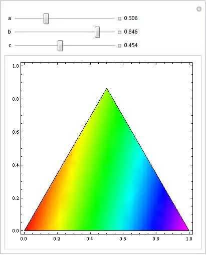
With another Manipulate, you can visualize the behaviour of your function (f here) depending on the values of a, b and c:

Manipulate[
 Dynamic@DensityPlot[f@trans@{x, y}, {x, 0, 1}, {y, 0, 1}, 
   ColorFunction -> (Hue[0.85 #] &), BoundaryStyle -> Black,
   RegionFunction -> (inQ@transform@{#1, #2} &)],
 {{a, 1., "a"}, 0, 1, Appearance -> "Labeled"},
 {{b, .5, "b"}, 0, 1, Appearance -> "Labeled"},
 {{c, .3, "c"}, 0, 1, Appearance -> "Labeled"},
 Initialization :> {
   x3 := (1 - x1 - x2),
   f[{x_, x2_, x3_}] := x a + x2 b + (1 - x - x2) c;
   inQ[pt_List] := (Total@pt == 1 && And @@ NonNegative@pt);
   trans[{x_, y_}] := {1, 0, 0} + x*{-1, 1, 0} + 
       y*{-1/Sqrt@3, -1/Sqrt@3, 2/Sqrt@3};
   }
 ]

Mathematica graphics

Thanks! That's the simplest method, I suppose. I like the disabled 3rd controller. — LBogaardt, Jan 19 '14 at 14:34

Manipulate Controller - Simplex

2 Answers2