I want to fit experimental data by the H-N model. Here is the H-N model: $$\text{EHN}(T)\text{=}\text{E$\infty $}+\frac{\text{E0}-\text{E$\infty $}}{\left(1+\left(i \omega\tau(T_g)10^{-\frac{\text{C1} (T-\text{Tg})}{\text{C2}+(T-\text{Tg})}}\right)^{\alpha }\right)^{\beta }}$$
Here is my data and code.
dataRe={{135., 2286.88}, {136., 1889.46}, {137., 1567.42}, {138.,
1294.73}, {139., 1081.55}, {140., 902.773}, {141., 761.623}, {142.,
643.534}, {143., 550.366}, {144., 470.925}, {145., 405.269}, {146.,
348.847}, {147., 303.248}, {148., 263.789}, {149., 230.926}, {150.,
202.368}, {151., 178.676}, {152., 158.557}, {153., 142.725}, {154.,
129.218}, {155., 118.192}, {156., 108.735}, {157., 101.272}, {158.,
94.8359}, {159., 89.3741}, {160., 84.4597}, {161., 80.1335}, {162.,
76.1632}, {163., 72.6128}, {164., 69.2969}, {165., 66.227}, {166.,
63.3502}, {167., 60.7664}, {168., 58.3432}, {169., 56.0645}, {170.,
53.8886}, {171., 51.8571}, {172., 49.9009}, {173., 48.014}, {174.,
46.1953}, {175., 44.4969}, {176., 42.8668}, {177., 41.3076}, {178.,
39.7966}, {179., 38.3511}, {180., 36.9621}, {181., 35.6673}, {182.,
34.4443}, {183., 33.3239}, {184., 32.2584}, {185., 31.245}, {186.,
30.2813}, {187., 29.4031}, {188., 28.5708}, {189., 27.781}, {190.,
27.0241}, {191., 26.3191}, {192., 25.6392}, {193., 24.975}, {194.,
24.3329}, {195., 23.7381}, {196., 23.1738}, {197., 22.6451}, {198.,
22.1308}, {199., 21.6239}, {200., 21.1439}, {201., 20.7245}, {202.,
20.3002}, {203., 19.8216}, {204., 19.3485}, {205., 18.9218}, {206.,
18.5166}, {207., 18.1276}, {208., 17.7492}, {209., 17.3845}, {210.,
17.0318}, {211., 16.6938}, {212., 16.3641}, {213., 16.0424}, {214.,
15.7233}, {215., 15.4063}, {216., 15.0967}, {217., 14.8008}, {218.,
14.5269}, {219., 14.2817}, {220., 14.0376}, {221., 13.7849}, {222.,
13.5334}, {223., 13.288}, {224., 13.0538}, {225., 12.831}, {226.,
12.6145}, {227., 12.4025}, {228., 12.1932}, {229., 11.9889}, {230.,
11.8003}, {231., 11.622}, {232., 11.442}, {233., 11.2606}, {234.,
11.0808}, {235., 10.9046}, {236., 10.7371}, {237., 10.577}, {238.,
10.4275}, {239., 10.2802}, {240., 10.1313}, {241., 9.98528}, {242.,
9.84445}, {243., 9.70511}, {244., 9.56583}, {245., 9.42439}, {246.,
9.28424}, {247., 9.16163}, {248., 9.05307}, {249., 8.94078}, {250.,
8.82361}, {251., 8.70563}, {252., 8.58908}, {253., 8.47813}, {254.,
8.37066}, {255., 8.26599}, {256., 8.16324}, {257., 8.06268}, {258.,
7.9627}, {259., 7.86389}, {260., 7.77106}, {261., 7.68272}, {262.,
7.59522}, {263., 7.50776}, {264., 7.4199}, {265., 7.33254}, {266.,
7.24746}, {267., 7.16453}, {268., 7.0849}, {269., 7.00582}, {270.,
6.92552}, {271., 6.84306}, {272., 6.76014}, {273., 6.68684}, {274.,
6.62505}, {275., 6.56069}, {276., 6.4861}, {277., 6.4139}, {278.,
6.34826}, {279., 6.28453}, {280., 6.2223}, {281., 6.16394}, {282.,
6.10795}, {283., 6.04993}, {284., 5.99424}, {285., 5.94735}, {286.,
5.90123}, {287., 5.84622}, {288., 5.78872}, {289., 5.74026}, {290.,
5.69521}, {291., 5.65082}, {292., 5.60682}, {293., 5.56378}, {294.,
5.52176}, {295., 5.48153}, {296., 5.44198}, {297., 5.40113}, {298.,
5.36029}, {299., 5.32389}, {300., 5.29061}, {301., 5.25599}, {302.,
5.22026}, {303., 5.18636}, {304., 5.15429}, {305., 5.12238}, {306.,
5.09002}, {307., 5.05626}, {308., 5.0215}, {309., 4.9884}, {310.,
4.95724}, {311., 4.9259}, {312., 4.89414}, {313., 4.86346}, {314.,
4.83431}, {315., 4.80636}, {316., 4.77938}, {317., 4.75121}, {318.,
4.72102}, {319., 4.69132}, {320., 4.66365}, {321., 4.63793}, {322.,
4.61535}, {323., 4.5939}, {324., 4.57255}, {325., 4.55129}, {326.,
4.53031}, {327., 4.50947}, {328., 4.48862}, {329., 4.46747}, {330.,
4.44536}, {331., 4.42347}, {332., 4.40477}, {333., 4.3878}, {334.,
4.36821}};
dataIm={{135., 887.339}, {136., 797.248}, {137., 701.968}, {138.,
608.569}, {139., 523.492}, {140., 445.966}, {141., 379.817}, {142.,
322.098}, {143., 274.838}, {144., 234.408}, {145., 201.682}, {146.,
173.669}, {147., 150.826}, {148., 130.956}, {149., 114.338}, {150.,
99.8744}, {151., 87.8489}, {152., 77.4709}, {153., 69.0043}, {154.,
61.7297}, {155., 55.8849}, {156., 50.8427}, {157., 46.6994}, {158.,
43.0493}, {159., 39.9282}, {160., 37.1165}, {161., 34.6505}, {162.,
32.3913}, {163., 30.3725}, {164., 28.5008}, {165., 26.8072}, {166.,
25.2321}, {167., 23.8052}, {168., 22.4737}, {169., 21.258}, {170.,
20.1175}, {171., 19.0709}, {172., 18.0847}, {173., 17.1751}, {174.,
16.3173}, {175., 15.5259}, {176., 14.7758}, {177., 14.076}, {178.,
13.4098}, {179., 12.7869}, {180., 12.1926}, {181., 11.6359}, {182.,
11.1054}, {183., 10.6106}, {184., 10.141}, {185., 9.7062}, {186.,
9.29656}, {187., 8.922}, {188., 8.57166}, {189., 8.25434}, {190.,
7.95882}, {191., 7.69154}, {192., 7.44172}, {193., 7.21152}, {194.,
6.99187}, {195., 6.78149}, {196., 6.57857}, {197., 6.38792}, {198.,
6.20788}, {199., 6.0449}, {200., 5.89388}, {201., 5.758}, {202.,
5.62656}, {203., 5.49434}, {204., 5.36374}, {205., 5.23765}, {206.,
5.11653}, {207., 5.00326}, {208., 4.89584}, {209., 4.79588}, {210.,
4.70075}, {211., 4.61033}, {212., 4.52086}, {213., 4.43049}, {214.,
4.33572}, {215., 4.23482}, {216., 4.13749}, {217., 4.04895}, {218.,
3.96654}, {219., 3.89063}, {220., 3.81765}, {221., 3.74721}, {222.,
3.67986}, {223., 3.61563}, {224., 3.55026}, {225., 3.48314}, {226.,
3.41624}, {227., 3.34984}, {228., 3.28314}, {229., 3.2159}, {230.,
3.14784}, {231., 3.08}, {232., 3.01543}, {233., 2.95542}, {234.,
2.90456}, {235., 2.85808}, {236., 2.81372}, {237., 2.76943}, {238.,
2.72368}, {239., 2.67735}, {240., 2.6309}, {241., 2.58498}, {242.,
2.54007}, {243., 2.49639}, {244., 2.45405}, {245., 2.41249}, {246.,
2.37127}, {247., 2.32927}, {248., 2.28662}, {249., 2.24441}, {250.,
2.20277}, {251., 2.16184}, {252., 2.12168}, {253., 2.0829}, {254.,
2.04515}, {255., 2.00862}, {256., 1.97252}, {257., 1.93656}, {258.,
1.90105}, {259., 1.8665}, {260., 1.83418}, {261., 1.80359}, {262.,
1.77372}, {263., 1.74444}, {264., 1.71617}, {265., 1.68854}, {266.,
1.66149}, {267., 1.63461}, {268., 1.60756}, {269., 1.5805}, {270.,
1.55363}, {271., 1.52752}, {272., 1.50251}, {273., 1.47878}, {274.,
1.45619}, {275., 1.43259}, {276., 1.40649}, {277., 1.38075}, {278.,
1.35628}, {279., 1.33193}, {280., 1.30753}, {281., 1.28371}, {282.,
1.26006}, {283., 1.23519}, {284., 1.21085}, {285., 1.18961}, {286.,
1.16996}, {287., 1.15244}, {288., 1.13717}, {289., 1.12452}, {290.,
1.11253}, {291., 1.10009}, {292., 1.08708}, {293., 1.07289}, {294.,
1.05803}, {295., 1.04329}, {296., 1.02881}, {297., 1.01485}, {298.,
1.00133}, {299., 0.98825}, {300., 0.97555}, {301., 0.96326}, {302.,
0.95127}, {303., 0.93939}, {304., 0.92759}, {305., 0.91595}, {306.,
0.90446}, {307., 0.89313}, {308., 0.88195}, {309., 0.87097}, {310.,
0.86024}, {311., 0.84998}, {312., 0.84021}, {313., 0.83063}, {314.,
0.82119}, {315., 0.81193}, {316., 0.80287}, {317., 0.79377}, {318.,
0.78453}, {319., 0.77542}, {320., 0.76659}, {321., 0.75783}, {322.,
0.74902}, {323., 0.74036}, {324., 0.73211}, {325., 0.72417}, {326.,
0.71666}, {327., 0.70927}, {328., 0.70162}, {329., 0.69383}, {330.,
0.68607}, {331., 0.67845}, {332., 0.67127}, {333., 0.66448}, {334.,
0.65796}};
EHN[T_] := E\[Infinity] + (E0 - E\[Infinity])/(1 + (I \[Omega] 10^(-((C1 (T - T0))/(C2 + (T - T0)))))^\[Alpha])^\[Beta];
fitRe=FindFit[dataRe,Re[EHN[T]],{{\[Alpha], 0.2}, {\[Beta], 0.6}, {E0, 4}, {E\[Infinity], 8000}, {C1,
17}, {C2, 50}, {\[Omega], 10}}, {T}}];
fitIm=FindFit[dataIm,Im[EHN[T]],{{\[Alpha], 0.2}, {\[Beta], 0.6}, {E0, 4}, {E\[Infinity], 8000}, {C1,
17}, {C2, 50}, {\[Omega], 10}}, {T}}];
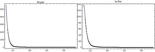
Show[ListPlot[dataRe, PlotStyle -> Red], Plot[Re[EHN[T]] /. {fitRe}, {T, 1, 200}]]
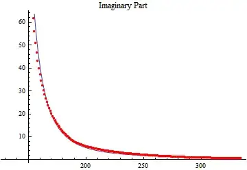
Show[ListPlot[dataIm, PlotStyle -> Orange], Plot[Im[EHN[T]] /. {fitIm}, {T, 1, 250}]]
However,I cannot fit the Real part and the Imaginary part well.Here is one of my fitted picture:

Is there any method,which I can fit both the Re and Im part. Thanks.


T0. – Kuba Jan 28 '14 at 08:39