Edit
I edited to replace h with N@h as suggested by MichaelE2, to prevent Mathematica slowdown if exact h is provided by the user.
Note for future users: I initially had a procedural approach posted, if you're interested in that method see the edit history.
I present a Functional approach, this is Mathematica after all.
SetAttributes[eulerMethod, HoldAll];

eulerMethod[func_, {x_, x0_, xmax_}, {y_, y0_}, h_] :=
 Module[{EulerStep, hh = N@h},
  EulerStep[{xi_, yi_}] := Module[{xold = xi, yold = yi, xnew, ynew},
    xnew = xold + hh;
    ynew = yold + hh ReleaseHold[Hold[func] /. {HoldPattern[x] -> xold,
          HoldPattern[y] -> yold}]; {xnew, ynew}];
      NestList[EulerStep, {x0, y0}, Round[(xmax - x0)/hh]
     ]
  ]
Usage
sol = eulerMethod[y^2 + t^2 - 1, {t, -2, 2}, {y, -2}, 0.2];
You can compare it to the built in NDSolve by plotting both in the range [-2, 2]
ListLinePlot[sol, Filling -> Axis]

For NDSolve:
nd = NDSolve[{y'[t] == y[t]^2 + t^2 - 1, y[-2] == -2}, y[t], {t, -2, 2}];
Then
Plot[y[t] /. nd, {t, -2, 2}, Filling -> Axis]
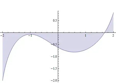
Clearly, our eulerMethod needs more iteration (smaller step size) to get close to the more accurate NDSolve
If we increase the number of iterations (decrease h) we nail the accuracy
sol2 = eulerMethod[y^2 + t^2 - 1, {t, -2, 2}, {y, -2}, 0.01]

ListLinePlot[sol2, PlotStyle -> {Red, Thick}, Filling -> Axis, FillingStyle -> Darker@Green]

Clearly, this looks very much like the result from NDSolve
You can get an exact solution using DSolve as follows:
DSolve[{y'[t] == y[t]^2 + t^2 - 1, y[-2] == -2}, y[t], t]
DSolvein the documentation centre. – Sektor Feb 06 '14 at 04:50