How to optimally solve and generalize this Conway's Game of Life puzzle

Question

I tried solving this using mma. I am aware of this command - Cellular automata. But i don't want to use that coz then there is no challenge. So below is how i did it and my question is can this be done with fewer lines of code (without resorting to CellularAutomaton). Also i wanted to generalize it to any initial condition.

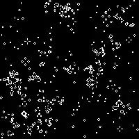
I am representing the grid shown in the puzzle as a (n $\times$ m) matrix such that all the live cells are represented by 1 and the dead ones by 0. Also in this particular case we have $n = 26$ and $m = 27$. Then i manually made a list of the initial condition given in the question. Here each pair represents the $(ij)^{th}$ element having live cells.

• [as a side note - can this process be automated - i mean finding this list from that image given for the intial grid by some image processing]

list = {{2, 6}, {2, 13}, {3, 23}, {3, 25}, {4, 3}, {4, 10},
       {4, 9}, {4, 18}, {5, 18}, {5, 2}, {8, 11}, {8, 12},
        {10, 10}, {10, 12}, {11, 11}, {12, 18}, {13, 2}, {14, 2}, {13, 
         23}, {14, 8}, {14, 23}, {16, 24}, {17, 25}, {18, 24},
          {18, 18}, {18, 17}, {19, 12}, {20, 12}, {20, 3}, {20, 4}, {22, 
        24}, {23, 23}, {22, 17}, {23, 18}};

The matrix $A_{n \times m}$ now contains the elements 1 and 0 corresponding to the live and dead cells receptively.
$f^{ij}_{0}$ contains the $(ij)^{th}$ element of $A_{n \times m}$

  A[n_, m_] := SparseArray[# -> 1 & /@ list, {n, m}, 0]

 Table[f[0][i, j] = A[26, 27][[i, j]], {i, 1, 26}, {j, 1, 27}];

The recursive function which gives the next generation is:-

f[k_][i_, j_] := f[k][i, j] = Module[{n = 26, m = 27, neg},

  findNeighbours[i, j] := Module[{},
     f[k - 1][#[[1]], #[[2]]] & /@ {{i - 1, j - 1}, {i - 1, 
       j}, {i - 1, j + 1}, {i, j - 1}, {i, j + 1}, {i + 1, 
         j - 1}, {i + 1, j}, {i + 1, j + 1}}];

   neg = Cases[findNeighbours[i, j], _Integer];

    (* Apply the rules to the ij th element*)
    Which[f[k - 1][i, j] == 1,
          Which[Count[neg, 1] < 2, 
          val = 0, (Count[neg, 1] === 2 || Count[neg, 1] === 3), val = 1, 
           Count[neg, 1] > 3, val = 0],
            f[k - 1][i, j] == 0,
            Which[Count[neg, 1] === 3, val = 1, True, val = 0]]

       ]

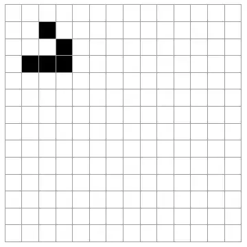
Finally we can plot the results to see the answer which is 3 if the starting generation is called $1^{st}$ generation.

   genaration[0] = 
     ArrayPlot[
    Table[f[0][i, j] = A[26, 27][[i, j]], {i, 1, 26}, {j, 1, 27}], Mesh -> True];


   genaration[n_] := 
     ArrayPlot[Table[f[n][i, j], {i, 1, 26}, {j, 1, 27}], Mesh -> True]

  res = ListAnimate[genaration[#] & /@ Range[0, 3], 
         AnimationRate -> 0.5]

Answer 1

My "Game of Life" implementation:

a = RandomInteger[BernoulliDistribution[0.1], {200, 200}];

Dynamic[Image[a =
   1 - Unitize[(# - 3) (# - 12) (# - 13)] &@
    ListConvolve[{{1, 1, 1}, {1, 10, 1}, {1, 1, 1}}, a, {2, 2}, 0]
  ]]

To use the initial grid in the question you would just initialise a with:

a = SparseArray[list -> 1]

However my code continuously updates the grid (quite rapidly), so the grid evolves to the "all dead" state in a fraction of a second.

To actually answer the question "how many generations have any life in them" you could write the evolution step as a function and use FixedPointList to count the number of steps:

evolve[a_] := 1 - Unitize[(# - 3) (# - 12) (# - 13)] &@
  ListConvolve[{{1, 1, 1}, {1, 10, 1}, {1, 1, 1}}, a, {2, 2}, 0]

Length@FixedPointList[evolve, Normal[SparseArray[list -> 1]]] - 2
(* 3 *)

Note that FixedPointList will generate the complete list of grids, so for larger problems you would want to use a different approach to avoid eating all your computer's memory.

Answer 2

This is one way of implementing Conway's Game of Life:

step[matrix_] := Module[{m = matrix, neighbours},
  neighbours = ListConvolve[{{1, 1, 1}, {1, 0, 1}, {1, 1, 1}}, ArrayPad[m, 1]];
  m = ReplacePart[m, Position[neighbours, _?(# == 1 || # > 3 &)] -> 0];
  m = ReplacePart[m, Position[neighbours, 3] -> 1]
  ]

For example, this is the so called glider:

m = ArrayPad[{{0, 1, 0}, {0, 0, 1}, {1, 1, 1}}, {1, 10}];
ListAnimate[ArrayPlot[#, Mesh -> True] & /@ NestList[step, m, 30]]

I've written about another cellular automata problem here and this includes a link to a post where image processing was used in Mathematica to get initial states for a cellular automata problem, so the answer to that question is that yes it is possible.