Perhaps this (an example):
Needs["ErrorBarPlots`"]
ErrorListPlot[{{{1, 1}, ErrorBar[0.2, 0.3]}, {{2, 2},
   ErrorBar[0.2, 0.3]}, {{3, 4}, ErrorBar[0.2, 0.5]}, {{4, 8},
   ErrorBar[1, 2]}},
 ErrorBarFunction ->
  Function[{coords, errs}, {Opacity[0.2],
    Disk[coords, {(errs[[1, 2]] - errs[[1, 1]])/
       2, (errs[[2, 2]] - errs[[2, 1]])/2}]}],
 PlotRange -> {{0, 6}, {0, 10}}, AspectRatio -> Automatic]
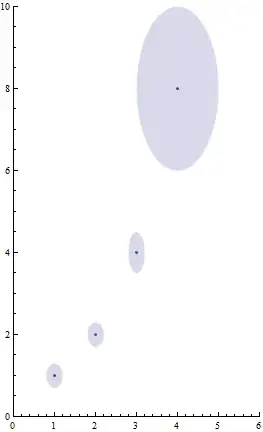
(aspect ratio to facilitate interpretation of error bars)
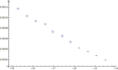
UPDATE
As per request (and limited due to major time pressures): a quickly devised answer based on data provided. Note I accept aim is visualization of y uncertainty by size of blob but uncertainty in 'x' whatever x is suggested.
data = {{-19.1651, 0.00313089, 2.4711*10^-6}, {-18.7084, 0.00311717,
    2.61428*10^-6}, {-18.2809, 0.00310325, 2.66765*10^-6}, {-17.8611,
    0.00309356, 2.54845*10^-6}, {-17.4091, 0.00308763,
    2.39272*10^-6}, {-17.0344, 0.00307304, 3.08935*10^-6}, {-16.5881,
    0.00306513, 2.9771*10^-6}, {-16.1826, 0.00305374,
    2.74635*10^-6}, {-15.7639, 0.00304204, 1.22568*10^-6}, {-15.3411,
    0.00303553, 1.4538*10^-6}, {-14.9394, 0.00302755,
    1.23145*10^-6}, {-14.5087, 0.00301919, 1.14451*10^-6}, {-14.1032,
    0.00300701, 1.00403*10^-6}};
datam = {{#1, #2}, ErrorBar[0, #3]} & @@@ data;

ErrorListPlot[datam,
 ErrorBarFunction ->
  Function[{coords, errs}, {Opacity[0.2],
    Disk[coords, {0.07, (errs[[2, 2]] - errs[[2, 1]])/2}]}],
 ImageSize -> 500]
The $r_x$ size was a guess...you could customize...currently do not have time.
Graphicsand place aDiskat the data point with the standard deviation as the radius. Example:Graphics[Disk[{##2}, #/20] & @@@ RandomReal[1, {10, 3}]]Don't usePlotMarkers, as their sizing is fickle, as you realized. – rm -rf Feb 18 '14 at 06:39ErrorBarFunctionis not the case with relative scalling. Where did you stuck in this, could you share any code you want to improve? – Kuba Feb 18 '14 at 07:26