MATLAB to Mathematica: coneplot

Question

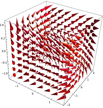
Does Mathematica have a function, similar to the one called coneplot in MATLAB? Given some spatial coordinates $x, y, z$ and velocity components $v_x,v_y,v_z$, it is able to produce the following graphs:

coneplot

When I plot my data with ListVectorPlot3D, I don't get any arrows shown. Here is a sample data, in the form $((x,y,z),(v_x,v_y,v_z))$:

data={{{0., 0.847912, 9.48902}, {0., 0., 0.}}, {{0.00773322, -0.0110065, 
   9.09927}, {0., 0., 0.}}, {{-1.00008, -0.0623481, 9.49984}, {0., 0.,
    0.}}, {{0., 0.847912, 10.8969}, {0., 0., 0.}}, {{0., 0.847912, 
   12.5007}, {0., 0., 0.}}, {{0., 0.847912, 14.1046}, {0., 0., 
   0.}}, {{0., 0.847912, 15.5729}, {0., 0., 0.}}, {{0., 0.847912, 
   16.6107}, {0., 0., 0.}}, {{0., 0.847912, 17.3334}, {0., 0., 
   0.}}, {{0., 0.847912, 18.0983}, {0., 0., 0.}}, {{0., 0.847912, 
   18.8639}, {0., 0., 0.}}, {{0., 0.847912, 19.9409}, {0., 0., 
   0.}}, {{0., 0.847912, 21.3189}, {0., 0., 0.}}, {{0., 0.847912, 
   22.822}, {0., 0., 0.}}, {{0., 0.847912, 24.6036}, {0., 0., 
   0.}}, {{0., 0.847912, 26.2343}, {0., 0., 
   0.}}, {{-1.08457, -0.0217237, 10.6779}, {0., 0., 
   0.}}, {{-1.11085, -0.0731095, 12.19}, {0., 0., 
   0.}}, {{-1.1131, -0.0651947, 13.7893}, {0., 0., 
   0.}}, {{-1.10496, -0.0720509, 15.108}, {0., 0., 
   0.}}, {{-1.12255, -0.0365039, 16.0888}, {0., 0., 
   0.}}, {{-1.12699, -0.00227834, 16.8818}, {0., 0., 0.}}, {{-1.15057,
    0.0126093, 17.6497}, {0., 0., 0.}}, {{-1.13931, -0.015588, 
   18.4211}, {0., 0., 0.}}, {{-1.03192, -0.0742988, 19.1016}, {0., 0.,
    0.}}, {{-1.24186, -0.0317904, 19.9972}, {0., 0., 
   0.}}, {{-1.14942, -0.0360112, 20.9677}, {0., 0., 
   0.}}, {{-1.09896, -0.0167395, 21.9511}, {0., 0., 
   0.}}, {{-1.117, -0.0452791, 23.2337}, {0., 0., 
   0.}}, {{-1.1522, -0.056303, 24.8936}, {0., 0., 
   0.}}, {{-1.09607, -0.110654, 26.195}, {0., 0., 
   0.}}, {{0.103537, -0.0647147, 26.6637}, {0., 0., 0.}}, {{0., 
   0.847912, 41.3051}, {0., 0., 0.}}, {{-0.012139, -0.0295375, 
   40.9221}, {0., 0., 0.}}, {{-0.857944, -0.0671514, 41.3642}, {0., 
   0., 0.}}, {{0., 0.847912, 42.4678}, {0., 4.67035*10^-7, 0.}}, {{0.,
    0.847912, 43.5378}, {0., 0., 0.}}, {{-0.979967, -0.033538, 
   42.2371}, {0., 0., 0.}}, {{-1.14769, -0.0351505, 43.0033}, {0., 0.,
    0.}}, {{-0.979351, -0.0342237, 43.8374}, {0., 0., 
   0.}}, {{-1.23767, -0.0499179, 44.5971}, {0., 0., 
   0.}}, {{-1.13972, -0.0000850668, 45.3128}, {0., 0., 
   0.}}, {{-1.12545, -0.00826265, 46.0778}, {0., 0., 
   0.}}, {{-1.1223, -0.0359113, 46.8929}, {0., 0., 
   0.}}, {{-1.12465, -0.055138, 47.8623}, {0., 0., 
   0.}}, {{-1.09846, -0.0144483, 49.0776}, {0., 0., 
   0.}}, {{-1.10899, -0.0625359, 50.4507}, {0., 0., 
   0.}}, {{-1.14579, -0.108309, 52.0417}, {0., 0., 
   0.}}, {{-1.12848, -0.01126, 54.0108}, {0., 0., 
   0.}}, {{-1.11299, -0.0970175, 55.2159}, {0., 0., 0.}}, {{0., 
   0.847912, 44.6206}, {0., 0., 0.}}, {{0., 0.847912, 45.3961}, {0., 
   0., 0.}}, {{0., 0.847912, 46.2075}, {0., 0., 0.}}, {{0., 0.847912, 
   47.3219}, {0., 0., 0.}}, {{0., 0.847912, 48.6172}, {0., 0., 
   0.}}, {{0., 0.847912, 50.0586}, {0., 0., 0.}}, {{0., 0.847912, 
   51.6502}, {0., 0., 0.}}, {{0., 0.847912, 53.7857}, {0., 0., 
   0.}}, {{0., 0.847912, 55.2595}, {0., 0., 
   0.}}, {{0.119852, -0.0804816, 55.6719}, {0., 0., 
   0.}}, {{1.38231, -0.0646805, 9.63683}, {0., 0., 
   0.}}, {{3.08676, -0.0356642, 10.2185}, {0., 0., 0.}}, {{3.98277, 
   0.0329428, 10.6312}, {0., 0., 0.}}, {{1.64587, 0.847912, 
   10.1128}, {0., 0., 0.}}, {{2.94532, 0.847912, 10.6054}, {0., 0., 
   0.}}, {{3.0844, 0.847912, 26.2343}, {0., 0., 0.}}, {{6.37314, 
   0.847912, 26.2343}, {0., 0., 0.}}, {{8.83598, 0.847912, 
   26.2343}, {0., 0., 0.}}, {{2.68672, -0.0254293, 26.6613}, {0., 0., 
   0.}}, {{5.13989, -0.0481681, 26.6588}, {0., 0., 
   0.}}, {{7.07074, -0.0263853, 26.6521}, {0., 0., 0.}}, {{8.87196, 
   0.0308362, 26.6941}, {0., 0., 0.}}, {{0.908045, -0.0256653, 
   41.2951}, {0., 0., 0.}}, {{0.90812, -0.0305627, 42.1266}, {0., 0., 
   0.}}, {{1.09331, -0.0723344, 42.9721}, {0., 0., 
   0.}}, {{1.03446, -0.06788, 43.5403}, {0., 0., 
   0.}}, {{1.9443, -0.0212229, 43.8278}, {0., 0., 0.}}, {{2.52323, 
   0.00655421, 44.1426}, {0., 0., 0.}}, {{1.47266, 0.847912, 
   44.0959}, {0., 0., 0.}}, {{1.47266, 0.847912, 44.6541}, {0., 0., 
   0.}}, {{3.48462, 0.847912, 55.2595}, {0., 0., 0.}}, {{9.45979, 
   0.847912, 55.2595}, {0., 0., 0.}}, {{15.9244, 0.847912, 
   55.2595}, {0., 0., 0.}}, {{20.8183, 0.847912, 55.2595}, {0., 0., 
   0.}}, {{24.5798, 0.847912, 55.2595}, {0., 0., 0.}}, {{27.9807, 
   0.847912, 55.2595}, {0., 0., 0.}}, {{4.19646, -0.079758, 
   55.6822}, {0., 0., 0.}}, {{9.8436, -0.111618, 55.6824}, {0., 0., 
   0.}}, {{17.6324, -0.0328765, 55.6789}, {0., 0., 
   0.}}, {{23.6589, -0.044735, 55.6773}, {0., 0., 
   0.}}, {{27.8005, -0.0722351, 55.6708}, {0., 0., 0.}}, {{2.94532, 
   0.847912, 11.1635}, {0., 0., 0.}}, {{2.62106, -0.0129568, 
   44.6594}, {0., 0., 0.}}, {{3.34577, -0.0199615, 44.9502}, {0., 0., 
   0.}}, {{3.9942, 0.0362858, 45.2367}, {0., 0., 0.}}, {{2.27968, 
   0.847912, 44.96}, {0., 0., 0.}}, {{2.94532, 0.847912, 
   45.2124}, {0., 0., 0.}}, {{2.94532, 0.847912, 45.7705}, {0., 0., 
   0.}}, {{4.30519, -0.0509312, 11.19}, {0., 0., 0.}}, {{5.04605, 
   0.847912, 11.9598}, {0., 0., 0.}}}

VectorPlot3D or ListVectorPlot3D with specyfic VectorStyle will give you cones. About the box: something like DensityPlot3D — Kuba, Mar 04 '14 at 09:35
@Kuba Please see my edit. I can't make it work with ListvectorPlot3D -- but I've added some of my data. — BillyJean, Mar 04 '14 at 09:59
@Kuba Hope it is fine now, please let me know if it is not. Really appreciate your help and time. — BillyJean, Mar 04 '14 at 10:11
Favorited, just to remind me to see what awesome solution Kuba & co. come up with... — ciao, Mar 04 '14 at 10:37
@mohsen This is just how my simulated data is (it's not random data) — BillyJean, Mar 04 '14 at 11:02
@BillyJean If they're all zeros then there's nothing to plot!! Of course it "doesn't work" with ListVectorPlot3D. All the vectors have zero length, and they're invisible. — Szabolcs, Mar 04 '14 at 14:21
While responding to @Szabolcs's comment, can you also specify what features are most important to you? Cones as arrows? Pretty specular cones? Cone sizes? pretty axes? If it is "all of the above", then at least prioritizing might help out a bit. — bobthechemist, Mar 04 '14 at 14:26
@Szabolcs Even if I use data=data+1, it still doesn't work. — BillyJean, Mar 04 '14 at 14:53
@bobthechemist If I can choose freely, then magnitude of the velocities is the most imporant -- i.e., is it possible to color them after their magnitude? — BillyJean, Mar 04 '14 at 14:53

bobthechemist · Answer 1 · 2014-03-04T18:33:45.187

Just tossing a thought out there. Using the following sample data from ListVectorPlot3D, Graphics directives can be applied to VectorStyle to get a shape you desire:

vectors = 
  Table[{{x, y, z}, {y, x - x^3, z}}, {x, -1.5, 1.5, 0.2}, {y, -2, 2, 
    0.2}, {z, -1, 1, 0.1}];
ListVectorPlot3D[vectors, VectorScale -> 0.05, 
 VectorStyle -> {Specularity[White, 20], Red, 
   Graphics3D[Cone[{{-2, 0, 0}, {1.5, 0, 0}}, 0.5]]}]

Mathematica graphics

Vector list plotting requires a structured grid of datapoints, otherwise the interpolation of the points fails and you get an empty plot without warning. Under circumstances where you cannot obtain data on a structured grid, creating a plot with graphics directives may be a better alternative.

Using your data = data + 1 option:

Graphics3D[{Specularity[White, 20], {ColorData["DarkRainbow"][Norm[#[[2]]]], 
  Cone[{#[[1]], #[[1]] + 1 + 1 #[[2]]}, 0.5 Norm[#[[2]]]]} & /@ data}, Axes -> True]

Mathematica graphics

Not a terribly pretty plot IMO, but I don't know what you are expecting from the sample data.

Thanks -- is there a way to do the same with the same format as my data? I know the velocities are zero, but say you use data=data+1 instead. — BillyJean, Mar 04 '14 at 15:24
@BillyJean your data fall on an unstructured grid, and the interpolation function used by ListVectorPlot3D is having troubles with that. If it is possible to generate the data on a structured grid, then you will run in to fewer problems. — bobthechemist, Mar 04 '14 at 16:46

MATLAB to Mathematica: coneplot

1 Answers1