How to numerically integrate this integral?

Question

I want to integrate a function (spherical coordinates):

$$\int _0^{2 \pi }\int _0^{\pi }\frac{r^2 \sin (\theta ) e^{-\lambda \sqrt{\rho ^2+r^2-2 \rho r \cos (\theta )}-2 r}}{\pi \epsilon \sqrt{\rho ^2+r^2-2 \rho r \cos (\theta )}}d\theta d\rho , ϵ=78.36, λ=0.548881$$

ϵ=78.36
λ=0.548881    
funcin = 
  1/(ϵ*π)*Exp[-(2*r + λ*Sqrt[r^2 + ρ^2 - 
    2*r*ρ*Cos[θ]])]*r^2*Sin[θ]*1/Sqrt[ρ^2 + r^2 - 2*r*ρ*Cos[θ]]
intfuncing = Integrate[funcin, {r, 0, Infinity}, {θ, 0, π}, {ϕ, 0,2 π}]

If I use analytic calculation (Integrate), an integral over r is left, which must be numerically evaluated, e.g., by using N[intfuncing] for specific ρ. For example I can write:

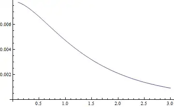
 Do[ρ = 0.1 + (i - 1)*0.05; int[[i]] = N[intfuncing], {i, 60}]

to calculate the integral at 60 points. But I get an error by that:

NIntegrate::slwcon: Numerical integration converging too slowly; suspect one of the following: singularity, value of the integration is 0, highly oscillatory integrand, or WorkingPrecision too small.

If I try to evaluate the integral numerically with NIntegrate, I get:

the integral ... evaluated to non-numerical values for all sampling points in the region with boundaries {{∞, 0.}, {0, 3.14159}, {0, 6.28319}}.

Does anyone have an idea how to solve this problem?

This is what I did, but the numerical integration gave the error with the convergence... — Guiste, Mar 04 '14 at 13:12
see here for the second error http://mathematica.stackexchange.com/questions/8899/how-do-i-prevent-nintegrateinumr-errors-within-other-functions, but really but really dont waste time with that if you can do it partially analytically — george2079, Mar 04 '14 at 13:13
note the original formulation actually works (I cant reproduce that error). Anyway its worth a note that its horrifically slow because N[Integrate[..]] re tries the analytic approach before evaluating numerically (x60...). Anybondy know the incantation to extract the arguments from an Integrate expression without evaluating it? (besides cut-paste! ) — george2079, Mar 04 '14 at 17:35

score 8 · Accepted Answer · answered Mar 04 '14 at 14:03

You can do the whole thing analytically:

(*ϵ=78.36;
λ=0.548881;*)
Clear[ϵ, λ];
funcin = 1/(ϵ * π) *
   Exp[-(2*r + λ * Sqrt[r^2 + ρ^2 - 2*r*ρ * Cos[θ]])] * r^2 * Sin[θ] *
    1 / Sqrt[ρ^2 + r^2 - 2*r*ρ * Cos[θ]];
intfuncinang = Assuming[r > 0 && ρ > 0 && ϵ > 0 && λ > 0,
  Integrate[funcin, {θ, 0, π}, {ϕ, 0, 2 π}]
  ]
(*
  -((2 E^(-2 r) (E^(-λ (r + ρ)) - E^(-λ Abs[r - ρ])) r)/(ϵ λ ρ))
*)

Assuming[ρ > 0 && ϵ > 0 && λ > 0,
  Integrate[intfuncinang, {r, 0, ρ}] + Integrate[intfuncinang, {r, ρ, Infinity}]
  ] // Simplify
(*
   (4 E^(-2 (1 + λ) ρ) (4 E^((2 + λ) ρ) + E^(2 λ ρ) (-4 + (-4 + λ^2) ρ))) /
     (ϵ (-4 + λ^2)^2 ρ)
*)

Good idea to separate the integration space, works out. – Guiste Mar 04 '14 at 16:36 — Guiste, Mar 04 '14 at 16:36

score 1 · Answer 2 · answered Mar 04 '14 at 13:55

You can do the integrals over the angular variables analytically; the result will be a function of r, ρ :

intth = 2 Pi Integrate[funcin, θ];
integ[ρ_] = (intth /. θ -> Pi) - (intth /. θ -> 0) ;

output = Table[{ρ, NIntegrate[integ[ρ], {r, 0, Infinity}]}, {ρ, 0.1, 3,0.05}] ;

ListLinePlot[output]

plot

How to numerically integrate this integral?

2 Answers2