5

My simple model is:

m[t_] := m[t] = m[t - 1]*p + 2
m[0] = 0
p = 0.5

I can plot the system as:

DiscretePlot[m[t], {t, 0, 50}]

Now, I would like to shock p for a short period, say, from 10 to 13 during which it would be 0.8 and then recovering its original value, 0.5, afterwards. Would Insert do this?

J. M.'s missing motivation
  • 124,525
  • 11
  • 401
  • 574
ppp
  • 817
  • 8
  • 15
  • 5
    I would guess something like 
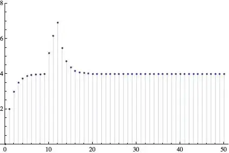
p[t_] /; 10 <= t <= 13 := 0.8; p[_] := 0.5. And use p[t] instead of p in your definition of m. But I don't understand the mathematical model. Could you explain it? – Michael E2 Mar 15 '14 at 20:13
  • @MichaelE2, thanks so much, I solved it! – ppp Mar 15 '14 at 23:50

2 Answers2

10

No, Insert wouldn't work in your case because m[t] isn't a List. In your recursive definition, the "shock" can be incorporated directly as follows:

Clear[m]; 
m[t_] := m[t] = m[t - 1]*Piecewise[{{q, 10 <= t <= 13}, {p, True}}] + 2
m[0] = 0;
p = 0.5;
q = 0.8;

DiscretePlot[m[t], {t, 0, 50}, PlotRange -> All]

DiscretePlot

What I did is use Piecewise to decide whether to apply the factor p or q.

Jens
  • 97,245
  • 7
  • 213
  • 499
2

As an alternative to Piecewise, you could construct a separate function for p using UnitStep. The modularity might provide more flexibility.

p[t_, shockAmplitudeDelta_, tBeginShock_, tEndShock_] := 0.5 + shockAmplitudeDelta(UnitStep[t - tBeginShock] - 
 UnitStep[t - tEndShock])
m[t_] := m[t] = m[t - 1]*p[t, 0.3, 10, 13] + 2
m[0] = 0;
DiscretePlot[m[t], {t, 0, 50}, PlotRange -> {0, 8}]

This provides the same DiscretePlot as Jens produced:

enter image description here

TransferOrbit
  • 3,547
  • 13
  • 26