14

I have a simple lattice / line manipulation:

Manipulate[r = 10; b = {{0, r}, {r, 0}};
l1 = Flatten[Table[i b[[1]] + j b[[2]], {i, 0, r}, {j, 0, r}], 1]/r;
Clear[a, b]; b = a /. Solve[a + y == 90, a][[1]]; x = y Pi/180;
g = Graphics[Line[{{0, 0}, {If[y <= 45, r/Cos[x], r/Cos[b Pi/180]], 0}}]];
rot = l : Line[pts_] :> Rotate[l, x, {0, 0}];
Show[Graphics[Point[l1], Frame -> True, AspectRatio -> 1], g /. rot], {{y, 45}, 0, 90}]

and would like to add points (that move with the manipulation) on the line that are perpendicular to the nearest points of the lattice, as shown below:

enter image description here

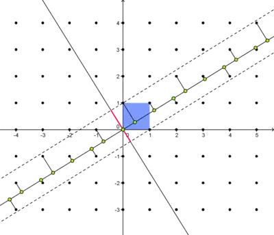
It would be a bonus if the perpendicular joining lines appeared also.

The only way I can think of pursuing this is to use something like Nearest, FrobeniusSolve, etc. (have been looking at the answers to this question with little success so far) to generate data for something along the lines of:

f = Graphics[Point[{{0, 0}, data, {If[y <= 45, r/Cos[x], 12], 0}}]];
rot1 = l : Point[pts_] :> Rotate[l, x, {0, 0}];
Show[Graphics[Point[l1], Frame -> True, AspectRatio -> 1], g /. rot, f /. rot1]

Note:

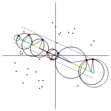
As noted by Vitaliy Kaurov below, the defining 'band' (dashed in the diagram) would not (necessarily) be symmetric about the main line. In this instance, the ratio of smaller to larger is the golden ratio. This is more obvious when looking at central red line in the above image - compare with:

enter image description here

I would ideally like this band width to be adjustable within the manipulation, but this is a minor concern.

Update

A minor modification of george2079's code

a = N[1/2 (Sqrt[(2/(5 + Sqrt[5]))] + Sqrt[10/(5 + Sqrt[5])])];
b = N[Sqrt[2/(5 + Sqrt[5])]];
Manipulate[Module[{grid, f, lndat, near, lnpts, lines1, lines2}, band = 1;
grid = Flatten[Outer[List, Range[-4, 4], Range[-4, 4]], 1];
f[x_] := m x;
lines1 = Select[pointlinedis[{{{0, 0}, {4, f[4]}}, grid}], 
Norm[Subtract @@ #] < a band &];
lines2 = Select[pointlinedis[{{{0, 0}, {4, f[4]}}, grid}], 
Norm[Subtract @@ #] < b band &];
Show[Plot[f[x], {x, -4, 4}, PlotRange -> 4], 
Plot[f[x] - b band/Cos[ArcTan[m]], {x, -4, 4}, PlotRange -> 4], 
Plot[f[x] + a band/Cos[ArcTan[m]], {x, -4, 4}, PlotRange -> 4], 
Graphics[{{Opacity[.5], PointSize[.015], Point[grid]},
{Orange, Thickness[.005], Line /@ lines1}, {Red, Opacity[.5], 
PointSize[.03], Point[#[[1]] & /@ lines1]}, {PointSize[.015], 
Blue, Point[#[[2]]] & /@ lines1}}], AspectRatio -> 1]], {{m, N[Pi/5]}, -10, 10}]
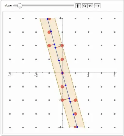
gives

enter image description here

which is nearly what I was after, but I would really like to exclude the points outside the lower line. If I swap lines1 for lines2 in bottom 3 lines of code, they are excluded, but so are some of points in top band. I have tried playing around with various If combinations, but can't seem to select points in upper band separately to points in lower band.

Also, point near $\{3,3\}$ shouldn't be included (though george2079 does note that this may happen in his answer).

martin
  • 8,678
  • 4
  • 23
  • 70
  • 1D quasicrystal with Fibonacci sequence of longer/shorter intervals ? – Vitaliy Kaurov Apr 08 '14 at 17:24
  • @Vitaliy Kaurov Yep, that's the one - but would like to create manipulation that shows what would happen where line is other than $\phi$. – martin Apr 08 '14 at 17:27
  • How you define the band of points which to select for perpendicular lines? – Vitaliy Kaurov Apr 08 '14 at 17:28
  • Ideally, that would be adjustable within the manipulation - sorry - forgot to add that in :/ - will correct in question. – martin Apr 08 '14 at 17:29
  • I don't think you put mathematical definition of bands - so no one understands what you need. If they are based on know golden ration distances you should explain that in the post. Or am I misunderstanding? – Vitaliy Kaurov Apr 08 '14 at 19:13
  • Bands are slightly different distances from main line (golden ratio in this case) - compare with central red line in image above. – martin Apr 08 '14 at 19:16
  • I would really like to be able to manipulate them separately though - (with default at golden ratio). – martin Apr 08 '14 at 19:17
  • I think nearest to a line points are defined without any band - they are actually the band. Are you saying you would like to expand the band to include not nearest points? – Vitaliy Kaurov Apr 08 '14 at 19:20
  • Yes - I suppose I am :/ ... sorry for not being clear!! :/ – martin Apr 08 '14 at 19:21
  • ... Nearest within a given tolerance value :/ – martin Apr 08 '14 at 19:21
  • 1
    for your asymmetric bands you need to select based on side, something like (Norm[Subtract @@ #] < b band && Det[{(Subtract @@ #), {4, f[4]}}] < 0 )& The sign of the determinant determines which side of the line. – george2079 Apr 10 '14 at 11:45

3 Answers3

12

So you guys know - quasicrystals are cool structures that can consist of finite number of parts which can be arranged in never repeating - aperiodic - pattern. Thing here is called projection method from a regular lattice.

http://www.nature.com/nmat/journal/v3/n11/fig_tab/nmat1244_F3.html

Interestingly if you know Fibonacci rabbits problem - that is also a 1D quasicrystal because sequence of 0 and 1 there is aperiodic.

Animate[
 Module[
  {grid, f, lndat, near, lnpts, lines, bnd1, bnd2},

  grid = Flatten[Outer[List, Range[-6, 6], Range[-6, 6]], 1];

  f[x_] := m x;

  lndat = 
   Select[{#, f[#]} & /@ Range[-6, 6, .01], -6 < #[[2]] < 6 &];

  near = Union[Flatten[Nearest[grid, #] & /@ lndat, 1]];

  lnpts = First[Nearest[lndat, #]] & /@ near;

  lines = Line /@ Thread[{near, lnpts}];

  {bnd1[x], bnd2[x]} = 
   m x + (#2 - 
        m #1) & @@@ (Sort[#, 
         EuclideanDistance @@ #1 > EuclideanDistance @@ #2 &] & /@ 
       GatherBy[
        Thread[{near, lnpts}], #[[1, 1]] - #[[2, 1]] > 0 &])[[All, 1, 
      1]];

  Show[
   Plot[Evaluate@{f[x], bnd1[x], bnd2[x]}, {x, -4, 4}, PlotRange -> 4,
     PlotStyle -> {Automatic, Dashed, Dashed}, 
    Filling -> {2 -> {3}}],
   Graphics[{
     {Opacity[.5], PointSize[.015], Point[grid]},
     {Red, Opacity[.5], PointSize[.03], Point[near]},
     {Orange, Thickness[.005], lines},
     {PointSize[.015], Blue, Point[lnpts]}}]
   , AspectRatio -> 1]
  ]
 , {{m, -4, "slope"}, -4, 4}, AnimationRunning -> False, 
 AnimationRate -> .5]

enter image description here

Vitaliy Kaurov
  • 73,078
  • 9
  • 204
  • 355
7

Here you are with the bands -- note also an (I think) improvement over the brute force fine discretization of the line: (I'm Not sure if that improved performance, but it didn't hurt and it looks cleaner)

caveat I think my little trick thinning down the lndat list is not guaranteed to find all of the strictly nearest points. It seems to work for the square grid but study that carefully if its critical.

 pointlinedis[{line_, pointlist_}] := 
     Module[{u = Subtract @@ line, mean = Plus @@ line/2},
        {#, (mean - u  #/2) &@(-(2 ( # - mean).u )/u .u) } & /@ pointlist ]
 Manipulate[Module[{grid, f, lndat, near, lnpts, lines},
   grid = Flatten[Outer[List, Range[-4, 4], Range[-4, 4]], 1];
   f[x_] := m x;
   lndat = pointlinedis[ {{{0, 0}, {4, f[4]}}, grid }][[;; , 2]];
   near = Union[Flatten[Nearest[grid, #] & /@ lndat, 1]];
   lines = pointlinedis[ {{{0, 0}, {4, f[4]}}, near }];
   zneg = Select[ lines , Det[{(Subtract @@ #), {4, f[4]}}] < 0 &];
   znegoff = Max[Norm[Subtract @@ #] & /@ zneg];
   zpos = Select[ lines , Det[{(Subtract @@ #), {4, f[4]}}] > 0 &];
   zposoff = Max[Norm[Subtract @@ #] & /@ zpos];
   Show[Plot[f[x], {x, -4, 4}, PlotRange -> 4],
        Plot[f[x] + {-znegoff , zposoff }/Cos[ArcTan[m]], {x, -4, 4}, PlotRange -> 4],
        Graphics[{{Opacity[.5], PointSize[.015], Point[grid]}, {Red, 
         Opacity[.5], PointSize[.03], Point[near]}, {Orange, 
         Thickness[.005], Line /@ lines}, {PointSize[.015], Blue, 
         Point[#[[2]]] & /@ lines}}], AspectRatio -> 1]], {{m, 1}, -7, 7}]

enter image description here

specified bands

It is actually a good bit simpler if you want to just specify the cutoff distance:

Manipulate[Module[{grid, f, lndat, near, lnpts, lines},
  band = 2;
  grid = Flatten[Outer[List, Range[-4, 4], Range[-4, 4]], 1];
  f[x_] := m x;
  lines = Select[ pointlinedis[{{{0, 0}, {4, f[4]}}, grid}], 
     Norm[Subtract @@ #] < band &];
  Show[
    Plot[f[x], {x, -4, 4}, PlotRange -> 4], 
    Plot[f[x] + {-band, band}/Cos[ArcTan[m]], {x, -4, 4}, PlotRange -> 4],
   Graphics[{{Opacity[.5], PointSize[.015], Point[grid]}, {Red, 
       Opacity[.5], PointSize[.03], Point[#[[1]] & /@ lines]}, {Orange,
       Thickness[.005], Line /@ lines}, {PointSize[.015], Blue, 
       Point[#[[2]]] & /@ lines}}], AspectRatio -> 1]], {{m, 1}, -7, 7}]

If you wanted both (true "nearest" and a cutoff) you can just use this lines=Select construct in the first example`

george2079
  • 38,913
  • 1
  • 43
  • 110
  • bands are great, but their respective distances from the main line would ideally be independently adjustable (so that one could be adjusted to be closer to the main line than the other) - thereby defining the nearest points within that specified tolerance band. The above example (and what Vitaliy Kaurov is referencing in his opening paragraph) is based on Fibonacci ratio - and defines the nearest points, rather than being a consequence of them. - See here. – martin Apr 08 '14 at 19:00
  • That is great - I will have a play with that & see if I can get them moving independently of one another :) – martin Apr 08 '14 at 19:29
  • Could you explain what pointlinedis does? – Vitaliy Kaurov Apr 08 '14 at 19:39
  • pointlinedis just finds the closest point on the line for each point in a list of points. – george2079 Apr 08 '14 at 19:51
  • @ george2079, I have updated question with slight modification to your code. Nearly there, but would appreciate it if you could cast your eye over it! :) – martin Apr 10 '14 at 10:04
4

Alternate answer, this is an exact analytic approach to the nearest point problem: (not i think precisely what @martin was after, but its an interesting problem and others may find it useful)

 lb = -1;ub = 1;
 pts0 = Select[Flatten[
   Table[ {i, j}, {i, 2 lb, 2 ub , .2}, {j, 2 lb , 2 ub , .2}], 1] ,Norm[#] < 1 &];
 intv[ p_, pn_] := 
 If[(pn[[1]] != p[[1]]),
    Piecewise[ {
       {Interval[{lb,  #}], pn[[1]] > p[[1]] &&  # > lb },
       {Interval[{ #, ub}], pn[[1]] < p[[1]] && # < ub},
       {Interval[], True}}] &@
            (  (pn + p).{1, #[[2]]/#[[1]] } &@(pn - p)/2 ),
    If[ p[[2]] <= pn[[2]], Interval[{lb, ub}], Interval[]]]
 Manipulate[
    pts = RotationMatrix[theta].# & /@ pts0;
    oo = First@Last@Reap[Do[(If[# =!= Interval[],
       Sow[{pts[[i]], #}]] &@
       (IntervalIntersection @@ (intv[pts[[i]], #] & /@ pts)))  ,
         {i, Length[pts]}]];
    band = Sort[oo[[;; , 1, 2]]][[{-1, 1}]];
    Show[Graphics[{Line[{{-1.25, 0}, {1.25, 0}}], 
                   Line[{{0, -1.25}, {0, 1.25}}],
             Rotate[{
              {Thick, Hue[RandomReal[{0, 1}]],
                 Line[{{#[[1]], 0}, {#[[2]], 0}}]} & /@
                   Partition[ Sort@Flatten[List @@ # & /@ oo[[;; , 2]]] , 2, 1],
              {Dashed, Line[{{lb, #}, {ub, #}}] & /@ band},
              {Red, PointSize[.02], Point[oo[[;; , 1]]]},
              {PointSize[.01], Point[pts]},
              {Line[{{#[[2, 1, 1]], 0}, #[[1]], {#[[2, 1, 2]], 0}}] & /@ oo}},
                -theta, {0, 0}]}]], {{theta, .1}, -2 Pi, 2 Pi}]

enter image description here

The color coding indicates the portions of the line that own each of the near points. (It would be trivial to show the perpendiculars as well but it gets a bit cluttered.)

A random point example:

enter image description here

enter image description here

george2079
  • 38,913
  • 1
  • 43
  • 110