Inhomogeneous phase-portrait with StreamPlot

Question

I have a problem with a must-be simple streamplot. The potential function governing the motion is U, and I have the following code in Mathematica:

U = -((1000.` x (1.25` - 1.` Sqrt[1 + 625.` x^2]))/Sqrt[1 + 625.` x^2])
StreamPlot[{Φ, -U}, {x, -0.05, 0.05}, {Φ, -1.5, 1.5}, StreamPoints -> Fine]

The problem is that I get the following plot: Wanna-be beautiful streamplot

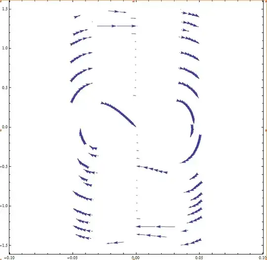
What did I do wrong, or how should I overcome this horror?

EDIT The result should look like the following phase plane plot created by MatLab: MatLab version

The MatLab code snippet:

f=@(Y) [Y(2); -1/2*Y(1)*(1000-1250/sqrt(1+625*Y(1)^2))];
y1=linspace(-0.06,0.06,20);
y2=linspace(-0.5,0.5,20);
[x,y]=meshgrid(y1,y2);

u=zeros(size(x));
v=zeros(size(y));

for i=1:numel(x)
    Yprime=f([x(i); y(i)]);
    u(i)=Yprime(1);
    v(i)=Yprime(2);
end

quiver(x,y,u,v,'r');
figure(gcf)
xlabel('x')
ylabel('xdot')
axis([-0.08 0.08 -0.6 0.6])

I used the same equation here, unfortunately due to the aspect ratio the arrows are a bit distorted.

I would like the Mathematica plot to have arrows 'all over the place' as in MatLab, so somehow the seeding should be altered. I would prefer the streamplot of mathematica rather than the MatLab version, as the StreamPlot shows the arrows along trajectories, whereas MatLab generates only a vectorfield.

a must-be simple streamplot. what does a simple streamplot mean? do you have an example of what the output is supposed to be from your book to compare? or explain more what is wrong with this. You need more lines? Scale is off? etc... — Nasser, Apr 19 '14 at 14:04
Can you please post the matlab code also? You can have an error in the translation. — Nasser, Apr 19 '14 at 15:39
the main problem is because of the plot ranges. If it is a diagonal shape with the same function, the resulted plot looks good. Unfortunately in that case the interesting phenomena cannot be seen, so we must use these border values — Adam, Apr 19 '14 at 15:45
I do understand your Matlab code here: You write f=@(t,Y) [Y(2); -1/2*Y(1)*(1000-1250/sqrt(1+625*Y(1)^2))]; but where is t in the RHS of the function f? Why are you defining f to accept (t,y) when t is not used in the function body? as for the main issue, I think one needs to understand your matlab code more to make sure what you are doing there and in Mathematica are mathematically equivalent. Having the Matlab code there helps. — Nasser, Apr 19 '14 at 16:21
you are right, 't' is not needed, I just used an old code for the plotting — Adam, Apr 19 '14 at 16:35
I believe this is the same problem I wrote about here. I guess at some point I should get around to implementing the solution I talked about in my answer. — , Apr 19 '14 at 17:46
I am afraid I will, but I still hope that someone will turn up here with a solution — Adam, Apr 19 '14 at 17:59
@Adam: I've implemented a solution in the previous answer. It works: http://i.stack.imgur.com/hOlpq.png — , Apr 21 '14 at 21:58

Inhomogeneous phase-portrait with StreamPlot

0 Answers0