Finding parameters making real part of eigenvalues vanish

Question

I have the following $\;3\times3$ matrix:

$\left( \begin{array}{ccc} 0.04 -0.4 b & 0 & 0.04 -0.4 b \\ 0 & -0.08-1.2 b & -0.06-0.9 b \\ 1.04 -0.4 b & 2.08 -0.8 b & 0 \end{array} \right)$

I want to find the $b$ values that make any of the eigenvalues of this matrix is $0$.

When I calculate the eigenvalues I get the following:

{Root[- 0.00832 - 0.0384 b + 1.264 b^2 - 0.48 b^3 + (0.08 + 2.24 b - 0.4 b^2) #1
      + (0.04 + 1.6 b) 2 + 1. #1^3&, 1], 
 Root[- 0.00832 - 0.0384 b + 1.264 b^2 - 0.48 b^3 + (0.08 + 2.24 b - 0.4 b^2) #1
      + (0.04 + 1.6 b) #1^2 + 1. #1^3&, 2],
 Root[- 0.00832 - 0.0384 b + 1.264 b^2 - 0.48 b^3 + (0.08 + 2.24 b - 0.4 b^2) #1
      + (0.04 + 1.6 b) #1^2+1. #1^3&, 3]}

Now I want to get the $b$ value that makes the real part of any of the eigenvalues $0$ with the following command:

Map[ NSolve[ Re[#] == 0 && b ∈ Reals, b] &, eigs]

Mathematica finds that the real part of the first eigenvalue will never be $0$, hence produces an empty set. However, for the roots $2$ and $3$, it does not evaluate the command. Also, first root is 0 when $b=0.1$ as I can see it in the plot below (red dots).

Is there any way to find $b$ more effectively?

Answer 1

Since Mathematica offers powerful symbolic capabilities I find that more effective solution to the problem uses exact numbers instead of machine precission ones and consequently exploits appropriate symbolic functions.

The given matrix m:

m = {{0.04 - 0.4 b, 0, 0.04 - 0.4 b}, 
     {0, -0.08 - 1.2 b, -0.06 - 0.9 b}, 
     {1.04 - 0.4 b, 2.08 - 0.8 b, 0}};

we rewrite it to exact (rational) numbers:

matrix = Rationalize @ m

{{  1/25 - (2 b)/5,                 0,   1/25 - (2 b)/5   }, 
 {               0, -(2/25) - (6 b)/5,  -(3/50) - (9 b)/10}, 
 { 26/25 - (2 b)/5,   52/25 - (4 b)/5,                   0} }

Now we can do simply this

sol = Solve[ Thread[ Eigenvalues[ matrix] == 0], b]

{{b -> -(1/15)}, {b -> 1/10}, {b -> 13/5}}

Instead of Thread[ Eigenvalues[matrix] == 0] one could write Eigenvalues[matrix] == {0, 0, 0}.

However this solution might be misleading since only one eigenvalue can vanish for every "solution" b while we explicitely required that all the eigenvalues vanish. Solve gives generic solutions (see e.g. What is the difference between Reduce and Solve?) thus if we are to find b when every eigenvalue vanishes then an appropriate approach exploits the MaxExtraConditions option of Solve or switches to Reduce:

Solve[ Thread[ Eigenvalues[matrix] == 0], b, MaxExtraConditions -> All]

{}

 Reduce[ Eigenvalues[matrix] == {0, 0, 0}, b]

False

In fact, one can be surprised that simple usage of Solve seemingly appears to be flawed, nevertheless the Root objects are responsible for this issue and basically it is an instance of inevitable operational incompatibility of different symbolic functions.

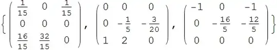
Now let's look at the output we can get with Solve:

matrixS = matrix /. sol;
MatrixForm /@ matrixS

and these are eigenvalues

 Eigenvalues /@ matrixS

 {{    1/30 (1 + Sqrt[65]),    1/30 (1 - Sqrt[65]),    0},
  { 1/10 (-1 + I Sqrt[29]), 1/10 (-1 - I Sqrt[29]),    0},
  {                -(16/5),                     -1,    0} }  

Edit

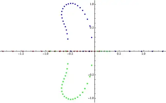
To underline that curious behaviour mentioned above let's consider eigenvalues in terms of Root[ poly[b], k] objects involving a parameter b with different numbers k. A critical issue is to realize that enumeration of roots depends on their values and may change when b changes. This plot clarifies the problem, here we use:

rt[k_] := Root[-26 - 120 b + 3950 b^2 - 1500 b^3 + (250 + 7000 b - 1250 b^2) #1 
               + (125 + 5000 b) #1^2 + 3125 #1^3 &, k] /. b -> x + I y /. x -> 1/10

Plot[ Re[ rt[#]& /@ {1, 2, 3}], {y, -1, 1}, Evaluated -> True, 
      PlotStyle -> Thickness[0.006], ImageSize -> 560, 
      PlotLegends -> Placed[Automatic, Below]]

The above problems may be prevented with ToRadicals, compare e.g.

Solve[ Root[-26 - 120 b + 3950 b^2 - 1500 b^3 + (250 + 7000 b - 1250 b^2) #1 
            + (125 + 5000 b) #1^2 + 3125 #1^3 &, 2] == 0, b]

{{b -> -(1/15)}, {b -> 1/10}, {b -> 13/5}} 

Solve[ ToRadicals[
         Root[-26 - 120 b + 3950 b^2 - 1500 b^3 + (250 + 7000 b - 1250 b^2) #1 
              + (125 + 5000 b) #1^2 + 3125 #1^3 &, 2]] == 0, b]

{}

Answer 2

Values of b for which real parts of eigenvalues vanish in fact make the imaginary parts also vanish. One can show this as follows.

m = Rationalize[{{0.04 - 0.4 b, 0, 
     0.04 - 0.4 b}, {0, -0.08 - 1.2 b, -0.06 - 0.9 b}, {1.04 - 0.4 b, 
     2.08 - 0.8 b, 0}}];
cp = CharacteristicPolynomial[m, z];

Replace z by x+I*y where we will look for only real values of x and y.

ee = Expand[cp /. z -> x + I*y];
polys = ComplexExpand[{Re[ee], Im[ee]}]

(* Out[103]= {26/3125 + (24 b)/625 - (158 b^2)/125 + (12 b^3)/25 - (2 x)/
  25 - (56 b x)/25 + (2 b^2 x)/5 - x^2/25 - (8 b x^2)/5 - x^3 + y^2/
  25 + (8 b y^2)/5 + 3 x y^2, -((2 y)/25) - (56 b y)/25 + (2 b^2 y)/
  5 - (2 x y)/25 - (16 b x y)/5 - 3 x^2 y + y^3} *)

We want to find values of b such that these polynomials, and x, all vanish. And we only count solutions for which y is real.

Select[{x, y, b} /. 
  Solve[Join[{x}, polys] == 0, {x, y, b}], Im[#[[2]]] == 0 &]

(* {{0, 0, -(1/15)}, {0, 0, 1/10}, {0, 0, 13/5}} *)

So there are only three values of b that make the eigenvalue real parts vanish, and they make the imaginary parts vanish as well.

Answer 3

An alternative is to recognize that the product of the eigenvalues is equal to the determinant. Hence:

m = {{0.04 - 0.4 b, 0, 0.04 - 0.4 b}, {0, -0.08 - 1.2 b, -0.06 - 0.9 b}, 
     {1.04 - 0.4 b, 2.08 - 0.8 b, 0}};
Roots[Det[m] == 0, b]

Since the Det is a 3rd order polynomial, there are three zeros, which occur when

b == 2.6 || b == 0.1 || b == -0.0666667