Plot A Function Of A Stochastic Process

Question

I am trying to do something very simple in Mathematica 9. I want to play around with option pricing and for that I thought it best to use the new stochastic process functionality.

So, first of all I simulate one instance of a geometric brownian motion:

$$ \frac{dX_t}{X_t} = \mu dt + \sigma dW_t\\ dW_t \sim N(0, 1) $$

Which in Mathematica is:

proc = ItoProcess[
   \[DifferentialD]x[t]/
    x[t] == σ \[DifferentialD]w[t] + μ \[DifferentialD]t, 
   x[t], 
   {x, x0},
   t,
   w \[Distributed] WienerProcess[]];

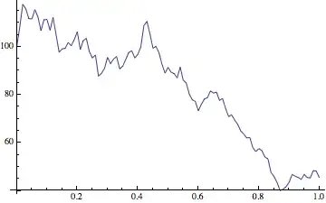
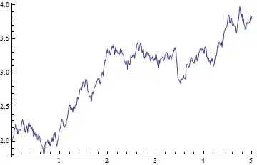
And here's an example of what I get, when I plot it, assuming $X_0 = 100$.

So, okay, when I create a plot of a RandomFunction of the process, then I actually plot the TemporalData for $X_t$ and not $dX_t$. Cool, whatever.

But now I want to plot, say $f(dX_t)$ or $f(X_t)$, where I would like to define $f$ as I see fit. And this is where I hit a brick wall. I have tried looking for hints in the docs or for answers here, but there are no definitive ones or the ones that seem to work.

I also feel, that I'm missing something fundamental here. Could somebody kindly suggest an answer or the venue of inquiry?

Answer 1

I'm not an expert on stochastic differential equations but I found the documentation clear enough.

Getting the output in terms of a function of your process variable x[t] is easy:

SeedRandom[1];
With[{σ = 1, μ = 1, x0 = 100},
  proc = ItoProcess[
           \[DifferentialD]x[t]/x[t] == σ \[DifferentialD]w[t] + μ \[DifferentialD]t, 
           Log10[x[t]], 
           {x, x0}, t, w \[Distributed] WienerProcess[]
         ];
 rp = RandomFunction[proc, {0., 5., 0.01}]
 ]

ListLinePlot[rp]

As you can see I changed x[t] as the output expression into Log10[x[t]].

The last line in the syntax block of the ItoProcess help page names the object in this location the "output expression". In the examples you usually see x[t] there, but it doesn't have to be just that.

A different route you could have traveled was using the TemoralData object that is being generated.

So if you start with just x[t] as output expression (as you originally did):

SeedRandom[1];
With[{σ = 1, μ = 1, x0 = 100},
  proc = ItoProcess[
           \[DifferentialD]x[t]/x[t] == σ \[DifferentialD]w[t] + μ \[DifferentialD]t, 
           x[t], {x, x0}, t, w \[Distributed] WienerProcess[]
         ];
 rp = RandomFunction[proc, {0., 5., 0.01}]
 ]
ListLinePlot[rp]

You can get the resulting path by getting the "Paths" properties from the TemporalData object:

rp["Paths"]

   (*==>  {{{0.`, 1.9999999999999998`}, {0.01`, 2.0247187089520158`}, 
           {0.02`, 2.0462858749445374`}, {4.97`, 3.811145935882086`}, 
            ...
           , {4.99`, 3.7933881925620243`}, {5.`, 3.826247092011493`}}} *)

You could use the function that you wanted to apply on this output:

ListLinePlot[MapAt[Log10, rp["Paths"], {All, All, 2}]]

which yields the same result as when the function is directly used as the output expression.