Solving a complex-valued differential equation with NDSolve

Question

I am trying to solve $dx/dt=\sqrt{1+(ix)^{1.8}}$ for initial condition $x[0] =-0.9877 + i 0.1563$, where $x$ is a complex variable. I would like to plot the imaginary part of the solution versus the real part. I used NDSolve and ParametricPlot.

s1 = 
  NDSolve[{x'[t] == (1 + (I x[t])^1.8)^0.5, x[0] == -0.9877 + I 0.1563}, x[t], {t, 0, 10}, 
    Method -> "ExplicitMidpoint", "StartingStepSize" -> 1/1000];

ParametricPlot[Evaluate[{Re[x[t]], Im[x[t]]} /. s1], {t, 0, 10}, 
  PlotRange -> Full, AspectRatio -> 1]

The result is wrong. I expect some kind of spiral. I think the problem is due to the fact that the graph crosses the branch cut which emanating from the origin. How can I fix it?

P.S.: I expect something like

enter image description here

It would be better if you add this to your earlier question here and provide some feedback to my answer there, if it wasn't clear. — Jens, Jun 07 '14 at 00:05
It was clear, but I was not looking for solving the DE with the direction fields. Eventually, I could solve the problem and obtained contours in a difficult way, by plotting many parts of the solution in different regions and stick all of them together. But here is a different situation. Because of non-integerity of 1.8 in the power, a new kind of branch cut appears... — , Jun 07 '14 at 05:21
I tried also by direction fields approach, again the answer is nonsense! — , Jun 07 '14 at 10:28
Dealing with branch-cuts can be difficult and NDSolve doesn't do it automatically. I don't understand what you expect we can do about it. — m_goldberg, Jun 07 '14 at 13:21
I am not restricted to NDSolve. Is there the any other approaches for plotting this? — , Jun 07 '14 at 14:44
@MichaelE2, hi sir, what do you think about this question : https://mathematica.stackexchange.com/questions/206901/plotting-ndsolve-function-in-complex-coordinates . Do you think it’s related? — S.S., Sep 26 '19 at 15:01

score 2 · Answer 1 · edited Apr 13 '17 at 12:56

Generically there are 10 branches to choose for the value of x'[t] at a value for x[t] in the OP's differential equation

deOP =    x'[t] == (1 + (I x[t])^(9/5))^(1/2)

In this form, however, there will be discontinuous jumps in the value of x'[t] whenever x[t] crosses a branch cut of the differential equation deOP. We can rationalize the equation to get the differential equation

deRat =   (x'[t]^2 - 1)^5 == (I x[t])^9

This form still has the intrinsic problem that there are generically 10 solutions for x'[t] for a given value of x[t]; however, there are not discontinuous jumps from crossing branch cuts in Mathematica functions.

Because of the square root (or equivalently, x'[t]^2), the roots come in pairs with opposite signs. The pair of integral curves corresponding to such a pair of roots in fact trace the same path in the complex plane, but in opposite directions. So generically through each value for x[0] pass five integral curves.

Theoretically the solutions may be computed with

NDSolve[{deRat, x[0] == x0}, x, {t, -8, 8}]

and indeed Mathematica tries to find all ten. It is slow and it seems to have trouble staying on the right branch (there are corners in the plots, indicating a discontinuity in the derivative).

Another approach is to differentiate deRat to get a second order equation that is linear in x''[t]; then x'[t] will be integrated from the initial value and Mathematica never has to choose a branch. The branch will be chosen by the choice of the initial value. If the initial value for x'[0] is dx0, then the following code will find the solution:

NDSolveValue[{
   x''[t] == (x''[t] /. First@Solve[D[deRat, t], x''[t]]),
   x'[0]  == dx0,
   x[0]   == x0},
  x, {t, -100, 100}] &,

The five initial values for x'[0] that yield the distinct integral curves may be found with

Select[
 x'[0] /. Solve[{deRat /. t -> 0, x[0] == x0}, {x[0], x'[0]}],
 Re[#] > 0 &]

Below I'll get all the solutions by mapping NDSolve over the initial values for x'[0]. I'll integrate each solution until it exceeds a specified distance from the initial point x[0], using WhenEvent. To plot the solutions, it will be convenient to change how the interpolating functions extrapolate, since each solution will have a different domain. The accepted answer to What's inside InterpolatingFunction[{{1., 4.}}, <>]? shows what parts of an InterpolatingFunction to modify to change the default extrapolation behavior. We can change the value returned by the InterpolatingFunction to Indeterminate; then ParametricPlot simply does not plot a point when the input t is outside of the domain. The function doNotExtrapolate alters an InterpolatingFunction in this way.

Here is the complete code:

ClearAll[x, t, doNotExtrapolate];
doNotExtrapolate[if_InterpolatingFunction] :=
  ReplacePart[if, {
    {2, 10} -> (Indeterminate &),      (* Extrapolation Handler *)
    {2, 2} -> 6                        (* Warning -> False *)
    }];


deOP = x'[t] == (1 + (I x[t])^(9/5))^(1/2);
deRat = (x'[t]^2 - 1)^5 == (I x[t])^9;

x0 = -9877/10000 + I  1563/10000;
plotradius = 10;
dx0All = SortBy[
   Select[
    x'[0] /. Solve[{deRat /. t -> 0, x[0] == x0}, {x[0], x'[0]}],
    Re[#] > 0 &],
   Arg[N[#]] &];

xAll = Map[
    NDSolveValue[{
       x''[t] == (x''[t] /. First@Solve[D[deRat, t], x''[t]]),
       x'[0]  == #,
       x[0]   == x0,
       WhenEvent[Abs[x[t] - x0] > plotradius, "StopIntegration"]},
      x, {t, -100, 100}] &,
    dx0All
    ] /. if_InterpolatingFunction :> doNotExtrapolate[if];

Output:

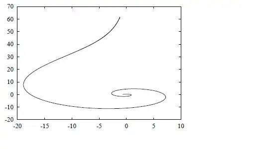
GraphicsRow @ Table[
  With[{dx = plotradius/n, plotctr = {-0.9877, 0.1563}},
   ParametricPlot[Evaluate[{Re[#[t]], Im[#[t]]} & /@ xAll], 
    Evaluate[{t}~Join~Through[{Min, Max}[Through[xAll["Domain"]]]]], 
    PlotRange -> (plotctr + {{-dx, dx}, {-dx, dx}}), 
    AspectRatio -> 1]
   ],
  {n, {1, 4, 50}}]

Mathematica graphics

Mathematica should add this as an example officially. Wonderful! — , Nov 21 '14 at 01:26

Solving a complex-valued differential equation with NDSolve

1 Answers1