0

There is an elegant way to obtain the envelope of an oscillation function explained here https://mathematica.stackexchange.com/a/27854/15966

My question is how to modify the code below so I can fit data to the obtained envelope with a parameter. How do I introduce a parameter into the module so it can be used later for fitting when the result of the module is an interpolation function.

Lets' generate some data

a = RandomReal[{20, 30}];  
b = RandomReal[{5, 10}];
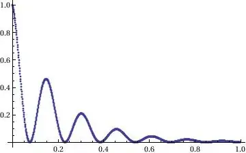
data = Table[{x, Cos[a*x]^2*Exp[-b*x]}, {x, 0, 1, 0.001}];
ListPlot[data, PlotRange -> All]

The code generates something like this:

data

Now the module below produces envelope for the given oscillating function

FunctionEnvelope[f_, {t_, a_, b_}, n_: 40] := 
 Module[{seeds, x, y, points, progress = 0, tempf, union}, 
  seeds = Rescale[Range[0, 1, 1/n] + 1/(2 n), {0, 1}, {a, b}];
  points = 
   Last[Last[
     Reap[Monitor[
       Do[Quiet@
         Check[progress++; {y, x} = FindMaximum[Abs[f], {t, x0}];
          x = t /. x; If[a <= x <= b, Sow[{x, y}]], Null], {x0, 
         seeds}], 
       ProgressIndicator[progress, {0, Length[seeds]}]]]]];
  union[] := 
   points = 
    Union[points, 
     SameTest -> (Abs[First[#1] - First[#2]]/
          Replace[Max[Abs[First[#1]], Abs[First[#2]]], 
           u_ /; u == 0 :> 1] < 10^-6 &)];
  union[];
  tempf = Interpolation[points];
  points = Quiet[Join[{{a, tempf[a]}}, points, {{b, tempf[b]}}]];
  union[];
  Interpolation[points]]

It can be used as follows:

q = 50;
f[t_] := E^(- 10*Abs[t]) * Cos[1000*t]/2 + 
  E^(-10*Abs[t])*Cos[(1000 + q)*t ]/2
g = FunctionEnvelope[f[x], {x, 0, 1}, 200];
Plot[{f[x], g[x]}, {x, 0, 1}, PlotRange -> All]

enter image description here

My question is how can I modify the module above to make it a function of the parameter q, so that the resulting interpolation function can be used to fit the data to get the optimal parameter q.

(The function f[t] is in principle can be moved to the definition of the module, I'm not going to change it.)

Thanks!

Mikayel
  • 551
  • 4
  • 8
  • Pretty sure the envelope of your function is just E^(-10 Abs[t]) Abs[Cos[q t/2]]. –  Jun 18 '14 at 09:30
  • Thank you for your reply. This is certainly true for the example. However, in general I'm going to have a function like this f[t_] := E^(- g1Abs[t]) Cos[1000*t]/2 + E^(-g2Abs[t])Cos[(1000 + q)*t ]/2 where g1 and g2 will have to be found to fit the initial data. I simplified it here for convenience, to understand how to insert a parameter into the definition of a module. – Mikayel Jun 18 '14 at 12:13

1 Answers1

4

still unclear what you are asking - is this close?

 f[q_, t_] := E^(-10*Abs[t])*Cos[1000*t]/2 + E^(-10*Abs[t])*Cos[(1000 + q)*t]/2
 g[qq_?NumericQ] := g[qq] = Evaluate[Block[{x}, FunctionEnvelope[f[qq, x], {x, 0, 1}, 200]]];

 Plot[{f[50, x], g[50][x]}, {x, 0, 1}, PlotRange -> All]

same as yours

 Plot[Table[g[q][x], {q, {2, 10, 50}}], {x, 0, 1}, PlotRange -> All]

enter image description here

edit

the is s useful thing to do whenever having issues with fitting parameters:

 Manipulate[
     Plot[g[q][x], {x, 0, 1}, PlotRange -> {0, 1}], {{q, 50}, 48, 52}]

If you run this you'll see the function jumps around somewhat erratically for small changes in the parameter. This is why you get an error " the gradient is larger than the tolerance " when running NonlinearModelFit

george2079
  • 38,913
  • 1
  • 43
  • 110
  • Thanks for the reply. I mean. that the command NonlinearModelFit[data, g[q][x], q, x] does not go, also for your definition of g[q]. – Mikayel Jun 19 '14 at 08:15
  • fix g to take only numeric arguments (see edit) then it works with NonlinearModelFit (crummy fit though if you mean to fit to the same data ) – george2079 Jun 19 '14 at 16:35
  • I guess it's crummy, because it does not work -). – Mikayel Jun 20 '14 at 08:13
  • I guess it's crummy, because it does not work -). Let's try data = Table[{x, Abs[Cos[44*x/2]]Exp[-10x]}, {x, 0, 1, 0.001}]; This generates data, that fits the envelope with q=44 very well (check Show[Plot[{g[44][x]}, {x, 0, 1}, PlotRange -> All, PlotStyle -> {Thick, Red}], ListPlot[data, PlotRange -> All]] ). If we now let NonlinearModelFit try to find it near q=40: nlm = NonlinearModelFit[data, g[q][x], {{q, 40}}, x] nlm["BestFitParameters"] with your new definition of g[q], it does not work: NonlinearModelFit::sszero: The step size in the search has become.. {q -> 41.} – Mikayel Jun 20 '14 at 08:21
  • 1
    it works in the sense that it is in a form suitable for input to NonlinearSolve. The fact you don't get a good result has to do with the behavior of your function, which is an entirely different issue. There are a bunch of questions on this site dealing with fitting difficulties. Typically you need to get very close with an initial guess at the solution. – george2079 Jun 20 '14 at 12:02