How to plot small values

Question

I wonder, why small values (eg. 10^-1600) would not show on a plot?

Here is a small example, where Evaluate gives a list of very small values and Plot does not show them, starting from x=20.

testfunc[x_] := 10^(-16 x) 
testvalues = {x -> {10, 20, 30, 40, 50, 60, 70, 80, 100}};
Evaluate[testfunc[x]] /. testvalues
LogPlot[Evaluate[testfunc[x]], {x, 1, 100}, AxesOrigin -> {0, 10^-1600}]

enter image description here

I guess it has something to do with precision, but I could not find any solution for Plot function yet and would appreciate any help. Had no luck with SetPrecision/WorkingPrecision.

Interestingly, with PlotRange -> All, the x-axis completely disappears... — Yves Klett, Jul 03 '14 at 18:28
Coincidentally :), $MinMachineNumber == 2.22507*10^-308. I suspect smaller numbers become 0. — Michael E2, Jul 03 '14 at 18:45
This gives the correct plot: LogPlot[Log@testfunc[x], {x, 1, 100}, WorkingPrecision -> $MachinePrecision]. It shouldn't, but it does. — Michael E2, Jul 03 '14 at 22:50
@MichaelE2 Why shouldn't it? Using $MachinePrecision will result in arbitrary precision. Perhaps you were thinking of MachinePrecision? Or do I misunderstand the implication of your comment? — Mr.Wizard, Jul 04 '14 at 04:50
@Mr.Wizard I misstated it: LogPlot[Log@testfunc[x], {x, 1, 100}, WorkingPrecision -> $MachinePrecision] gives the (correct) plot of LogPlot[testfunc[x], {x, 1, 100}] (V9.0.1, 8.0.4, 7). Log@testfunc[x] is negative over plot domain -- LogPlot should yield a blank graph. Right?? — Michael E2, Jul 04 '14 at 13:13
Btw, it doesn't matter what the working precision is, as long as it's about 4 or more. One can also compare with ListLogPlot[Table[Log@testfunc[x], {x, 1, 100}]] and ListLogPlot[Table[testfunc[x], {x, 1, 100}]]. The same thing happens with other underflow functions inside Log, AFAICT, e.g. LogPlot[Log[10^(-400) Sin[x]], {x, 0, 20}, WorkingPrecision -> $MachinePrecision]. — Michael E2, Jul 04 '14 at 13:32

score 6 · Accepted Answer · edited Jul 04 '14 at 04:34

Hm, probably the reason why you do not get the expected result is the values of x chosen for the Plot. As most likely they are chosen as Reals (which is connected with finite MachinePrecision), all of them will be zeros.

Consider the following simplification:

test = Map[10^(-16 #) &, Range[10, 100, 10]];
ListLogPlot[test]`
(*
   image generated with 
     ListLogPlot[test2, 
       Frame -> True, FrameLabel -> {"x", "testfunc(x)"}, 
       PlotMarkers -> Automatic, Joined -> True, 
       LabelStyle -> Directive[Black, FontSize -> 12], ImageSize -> 300]
 *)

example 1

Here we deal with infinite precision and everything is shown on the plot.

As Michael E2 noticed in his comment, even 10.^(-16 #) would work in the code above. The reason why this would work is that Mathematica switches to arbitrary-precision when dealing with numbers that can not be expessed with machine precision. LogPlot/Plot functions do not deal with arbitrary precision though (this is just an observation though).

Edit:

Check the code below:

test2=Reap[Plot[testfunc[x], {x, 0, 100}, 
 EvaluationMonitor :> Sow[{x, testfunc[x]}]];][[-1,   1]]; 
ListLogPlot[test2]
(*Reap and Sow allow to check which points were chosen by Plot function for plotting*)

example 2

Here we get the proper result as we get just the calculated values.

On the other hand, the FullForm function clearly shows that Plot disregards small numbers (which in most cases is understandable).

FullForm[Plot[testfunc[x] // sp, {x, 0, 100}]][[1, 1, 1, -1, -1,  1, ;; 10]]

(*This prints first ten points sampled by Plot.*)

This works with Map[10.^(-16 #) &, Range[10, 100, 10]], too, because the coordinates of ListLogPlot are the logarithms and Mma will switch to arbitrary precision numbers for higher values of 16 #, thus avoiding underflow. — Michael E2, Jul 03 '14 at 18:49
Indeed, ListLogPlot gives a proper result. Does it mean that there is no way to make Plot work with infinite precision? — megasplash, Jul 03 '14 at 19:11
Olga, I'd say (but I'm no expert) that since we do not have control over the sampling, it may be not possible to make LogPlot to work. I tried applying higher precision, but it failed to change anything. @Öskå, I'll do that:-). — Grzegorz Rut, Jul 03 '14 at 19:24

score 4 · Answer 2 · answered Jul 04 '14 at 00:10

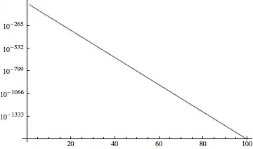
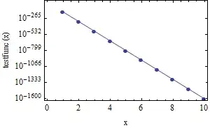
At some point, the plot functions make the coordinates machine-sized numbers. At that point, numbers smaller than [$MinMachineNumber](http://reference.wolfram.com/mathematica/ref/$MinMachineNumber.html) (`2.22507*10^-308` on my MacBook Pro) probably get converted to zero. `LogPlot` and `ListLogPlot` behave differently. It appears as if numbers less than `$MinMachineNumberare converted to zero byLogPlot**before** being plugged intoLog, whereasListLogPlottakes theLog` first.

Here's a workaround that allows one to use the sampling of Plot. Apparently, the underflow does not interfere with Plot's adaptive sampling.

ListLogPlot[
 Transpose[{#[[1]], Exp[#[[2]]]} &@Transpose[#]] & /@ 
  Cases[Plot[Log@testfunc[x], {x, 1, 100}], Line[pts_] :> pts, Infinity],
 Joined -> True]

Mathematica graphics

A general purpose function:

Options[listLogPlotFromPlot] = 
  DeleteDuplicates@Join[Options[ListLogPlot], Options[Plot]];
SetAttributes[listLogPlotFromPlot, HoldAll];

listLogPlotFromPlot[f_, domain_, opts : OptionsPattern[]] :=
 With[{plotopts = FilterRules[{opts}, Options[Plot]]},
  ListLogPlot[
   Transpose[{#[[1]], Exp[#[[2]]]} &@ Transpose[#]] & /@ 
    Cases[Plot[Log[f], domain, plotopts], Line[pts_] :> pts, Infinity],
   FilterRules[{opts}, Options[ListLogPlot]]
   ]
  ]

Unfortunately, separate Lines get styled with separate colors by ListLogPlot:

listLogPlotFromPlot[10^-400 Sin[x]^2, {x, 0, 16}]

Mathematica graphics

One can fix it by supplying a PlotStyle. Below we also join the points with a Line.

listLogPlotFromPlot[10^-400 Sin[x]^2, {x, 0, 16},
 Joined -> True, PlotStyle -> ColorData[1][1]

Mathematica graphics

One could also fix the coloring problem in the function listLogPlotFromPlot, but it seemed preferable to leave disconnected lines disconnected. Beware, there may be problems, especially with styling, if a list of functions is used. It would be best to generate the plots separately and combine with Show.

How to plot small values

2 Answers2

Linked