Backsubstituting solution into FindRoot and Plot

Question

I want to find roots from a transcendental equation using FindRoot as a function of a real parameter and then plot the solutions vs. the parameter. The following commands work perfectly:

equ[a_?NumericQ] := FindRoot[x == E^(-a x), {x, 1}][[1, 2]];

Plot[equ[a], {a, 0, 5}]

However, I actually have a much more complicated equation which is very sensitive on the starting value. Thus, starting from the second point, I want to set as the initial guess for each solution the value obtained on the previous point.

The trick proposed here works for a Table:

sol = {x -> 0};
sols = Table[sol = FindRoot[a x == 1, {x, sol[[1, 2]]}], {a, 1, 10}]

{{x -> 1.}, {x -> 0.5}, {x -> 0.333333}, {x -> 0.25}, {x -> 0.2}, {x -> 0.166667}, 
 {x -> 0.142857}, {x -> 0.125}, {x -> 0.111111}, {x -> 0.1}}

However, when I tried to plot the solutions I followed the suggestion here: plotting output from FindRoot

But the command

ListPlot[a /. sols]

only produced an empty graph.

So, how do I accomplish this?

I would rather be able to define a function of the roots in terms of the parameter a and then plot the function, but if I try something like

sol = {x -> 0};

equ[a_?NumericQ] := {sol = FindRoot[x == E^(-a x), {x, sol[[1, 2]]}]};

Plot[equ[a], {a, 0, 2}]

it will generate an empty plot again.

Answer 1

This is just another approach using NSolve rather than FindRoot. In the real domain this has a unique solution.

g[a_] := Quiet[x /. First@NSolve[x == Exp[-a x], x, Reals]];

You can plot:

Plot[g[u], {u, 1, 4}]

Tabulating makes processing faster, e.g.:

Manipulate[
 Plot[{x, Exp[-p x]}, {x, 0, 3}, PlotRange -> {0, 1}, 
  MeshFunctions -> (#1 - Exp[-#1 p] &), Mesh -> {{0.}}, 
  MeshStyle -> {Red, PointSize[0.02]}, 
  Epilog -> 
   Inset[Framed[
     ListPlot[tab, Joined -> True, 
      Epilog -> {Red, PointSize[0.04], Point[{p, g[p]}]}, 
      ImageSize -> 120]], {2, 0.68}]], {p, 1, 4, 
  Appearance -> "Labeled"}, 
 Initialization :> (tab = Table[{t, g[t]}, {t, 1, 4, 0.1}])]

Answer 2

thank you all for your suggestions.
They have been very helpful.

I concluded that by defining 2 functions, as in the following:

 x0 = {x -> 1};

 f1[a_?NumericQ] := {x0 = FindRoot[x == E^(-a x), {x, x0[[1, 2]]}]};

 f2[a_] := x /. f1[a];

I can Plot[f2[a],{a,0,2}] and obtain what I wanted.

Now, moving on to my real problem. What I really want to do is to find the complex roots of some very complicated equations, involving generalized hypergeometric and the Meijer G functions.

So, I first tried to solve a simpler, well-known equation, which provides the dispersion relation of longitudinal (a.k.a. Langmuir) waves in thermal plasmas.
The code I wrote is the following:

================================================

 ZF[z_] = I Sqrt[\[Pi]] E^-z^2 Erfc[-I z];

 Zp[z_] = -2 (1 + z ZF[z]);

 de[q_?NumericQ] := {z0 = FindRoot[2 q^2 - Zp[z/(Sqrt[2] q)], {z, z0[[1, 2]]}]};

 drl1[q_] := z /. de[q];

 drl2[q_?NumericQ] :=  FindRoot[2 q^2 - Zp[z/(Sqrt[2] q)], {z, 1}][[1, 2]];

================================================

The functions ZF[z] and Zp[z] evaluate the plasma dispersion (or Faddeeva) function and its derivative. The function de[q] implements the numerical solution of the dispersion equation. The function drl1[q] contains the dispersion relation, obtained with the "backsubstituting method" you helped me to implement. The function drl2[q] does the same, but the initial guess is fixed at z = 1.

When I plotted the real part of both drl1[q] and drl2[q] I got the following outputs:

=======================================

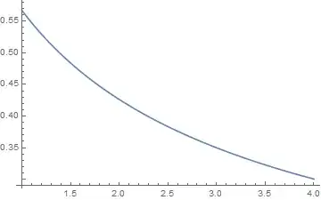
 Plot[Re[drl2[q]], {q, 0.01, 2}]

 z0 = {z -> 1};

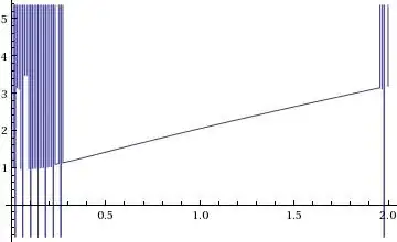
 Plot[Re[drl1[q]], {q, 0.01, 2}]

========================================

As you can see I got mixed results. Comparing both plot you can easily guess the correct curve. Now I guess that I either have an accuracy problem or I have to select and configure the appropriate method employed by FindRoot.

When I implement the same type of root-finding code in a FORTRAN program I always use the previous solution as the initial guess for the next one. That's why I wanted to do the same with Mathematica. Unfortunately, it didn't quite work out...

I naively tried to increase the working precision:

==============================================

 Plot[Re[drl2[q]], {q, 0.01, 2}, WorkingPrecision -> 48]

 z0 = {z -> 1};

 Plot[Re[drl1[q]], {q, 0.01, 2}, WorkingPrecision -> 48]

============================================

And it seems that the root-finder is jumping between 2 solutions.

Can you give me now some hint here? I confess that I'm not very savvy with Mathematica and don't really know which methods are implemented.

I've found a list in: here. Are those the methods I have at my disposal? Which one would be the best suited to find complex roots of transcendental functions?

In my FORTRAN codes I always use the Miller method because it's very simple and robust, but it seems that Mathematica does not support it.

Answer 3

sol = {x -> 0}; 
sols =  Table[sol = FindRoot[a x == 1, {x, sol[[1, 2]]}], {a, 1, 10}];
ListPlot[x /. sols]

sol = {x -> 0};
equ[a_?NumericQ] := {sol = FindRoot[x == E^(-a x), {x, sol[[1, 2]]}]};
Plot[x /. equ[a], {a, 0, 2}]

ListPlot[Flatten[Table[{a, x} /. equ[a], {a, 0, 2, .05}], 1]]