Problem with Poincare section

Question

these are equations for some double oscillators:

$x'(t)=p, p'(t)=-x-3y, y'(t)=q, q'(t)=-y-3x$

I would like to plot the Poincare section for collection of $(y,q)$ when $x=0$ and $x'(t)>0$ (or for $(x,p)$ when $y=0$ and $y'(t)>0$). I benefited from documentation and nice answer by Mr. belisarius here and I wrote:

abc = {x'[t] == p[t], p'[t] == -x[t] - y[t], y'[t] == q[t], q'[t] == -y[t] - x[t]};
psect[{x0_, p0_, y0_, q0_}] :=
Reap[NDSolve[{abc, x[0] == x0, p[0] == p0, y[0] == y0, q[0] == q0,
WhenEvent[x[t] + 0*y'[t] + 0*p[t] + 0*q[t] == 0,
If[p[t] >= 0, Sow[{y[t], q[t]}]]]}, {x, p, y, q}, {t, 0, 200},
MaxSteps -> \[Infinity], MaxStepSize -> .0005]][[2, 1]];
ps = psect /@ Table[{0.01, 0.005, 0.01, i}, {i, -.01, .01, .00125}];
ListLinePlot[#[[FindCurvePath[#][[2]]]] & /@ ps, Mesh -> All, PlotRange -> All]

But I don't receive anything. I expect to obtain something like this: enter image description here

Many thanks for your attention.

@belisarius Please, could you help me to figure out this problem? — Suzanne, Jul 14 '14 at 05:24

score 5 · Answer 1 · edited Jul 14 '14 at 09:53

This may simply be just an error in transcribing desired system for assessment. However, I post this to amplify Gregory Rut's answer for the coded system. Please note:

documentation of Poincare section uses well defined non-linear system with specific initial conditons. This is somewhat different to this system and what is being tabulated.
I am using the coupled linear system coded for and not the one in $\LaTeX$ which seems different (note the latter grows exponentially up very quickly, where as the former grow linearly ).
this system can be solved analytically and I exploit this for illustrative purposes (noting the similar pattern to Gregory Rut).
ideally I would have liked to place the axes labels. However, MMA10 seems to not do this well (I'd be interested in other users advice)

I have only plotted small t range (as solutions grow).

fun[a_, b_, c_, d_] := 
DSolve[{x'[t] == p[t], p'[t] == -x[t] - y[t], y'[t] == q[t], 
q'[t] == -y[t] - x[t], x[0] == a, y[0] == b, p[0] == c, 
q[0] == d}, {x[t], y[t], p[t], q[t]}, t]; 
tab =Table[{x[t], y[t], q[t]} /.First@fun[0.010, .01, 0.005, j], {j, -.01, .01, .00125}];

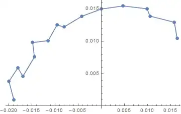
Plotting typical solutions with time (last entry of table):

enter image description here

Now, the table is a set of solutions for different initial conditions ($q(t)$). For any one solution you could section with perturbing initial condition ($q(t)$ which is y velocity) the following is an interactive example. I believe both the typical solution and the interactive approach illustrate the expected reason for small number of points: solutions leave space very quickly. I guess it gives insight as to how quickly solutions diverge with change in initial condition.

Manipulate[
 Show[ParametricPlot3D[Evaluate@tab[[1 ;; pl]], {t, 0, 30}, 
   PlotPoints -> 200, MeshFunctions -> {#1 &}, Mesh -> {{x0}}, 
   MeshStyle -> PointSize[0.02], LabelStyle -> 12, PlotStyle -> st], 
  ContourPlot3D[
   x == x0, {x, -0.06, 0.06}, {y, -0.08, 0.08}, {z, -0.08, 0.08}, 
   Mesh -> False, ContourStyle -> {Blue, Opacity[0.2]}], 
  ImagePadding -> 20, ImageSize -> 500, 
  PlotRange -> {{-0.06, 0.08}, {-0.06, 0.08}, {-0.08, 
     0.08}}], {st, {None, Automatic}}, {x0, -0.04, 0.04}, {pl, 
  Range[17]}, 
 Initialization :> (fun[a_, b_, c_, d_] := 
    DSolve[{x'[t] == p[t], p'[t] == -x[t] - y[t], y'[t] == q[t], 
      q'[t] == -y[t] - x[t], x[0] == a, y[0] == b, p[0] == c, 
      q[0] == d}, {x[t], y[t], p[t], q[t]}, t]; 
   tab = Table[{x[t], y[t], q[t]} /. 
      First@fun[0.010, .01, 0.005, j], {j, -.01, .01, .00125}];)]

enter image description here

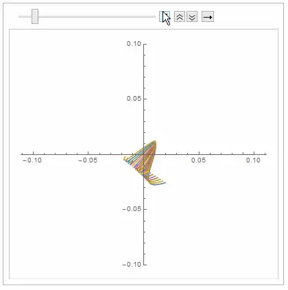
And similar insights are developed by just looking at x-y plane (with time) for the various initial conditions:

ListAnimate[
 Table[ParametricPlot[Evaluate@tab[[All, {1, 2}]], {t, 0, j}, 
   PlotRange -> {-0.1, 0.1}], {j, 1, 20}]]

enter image description here

@Suzanne I hope this is helpful..we all learn a lot from playing around...others may have better advice and insights. — ubpdqn, Jul 14 '14 at 06:55
But only a question, if I want to plot Poincare section for specified initial condition like the one in Documentation, what should I do? — Suzanne, Jul 14 '14 at 06:57
Could you add also the Poincare section plot for some specific initial values (as you wish), in your answer? — Suzanne, Jul 14 '14 at 07:00
@GregoryRut my sincerest apologies for incorrectly citing your name! Thank you for correcting! — ubpdqn, Jul 14 '14 at 09:57
@Suzanne I suggest you start by playing with your own code with one initial condition and noting the comments of Gregory Rut...just look at output, plot it etc. I have to help my partner with chores at the moment. Others may give you better advice also. Try for yourself...if you get stuck in a major way you can post a question with your new deliberations. — ubpdqn, Jul 14 '14 at 10:00

score 4 · Answer 2 · answered Jul 13 '14 at 22:07

It seems that you need to filter your results and select only numbers (some of points were not evaluated correctly)

sps = Flatten[Select[ps, NumberQ[#[[1, 1]]] &], 1];

Now the plot should be ok (note that there are very few points, you'd have to increase their number in order to get a better picture).

ListLinePlot[#[[FindCurvePath[#][[1]]]] &@sps, Mesh -> All, 
PlotRange -> All]

enter image description here

There's a small modification in your code needed: '/@'->'@'. '/@' is the same as Map whereas '@' calls an argument for a function, for instance Sin[x] is the same as Sin@x.

Problem with Poincare section

2 Answers2

Linked