Performing a chi-square goodness of fit test

Question

How would I perform a chi-square goodness of fit test? I have tried the following, where my data consists of the observed values whilst the data pair contains the correct values. Then I use the DistributionFitTest on the data and the data pair.

data = {115, 188, 97};
datapair = {100, 200, 100};
DistributionFitTest[datapair, data]

(* Out= 0.248213 *)

However the result I get is 0.248 and should be 0.216. Am I doing something wrong? And how would I measure the $\chi^2$ value?

Answer 1

The name PearsonChiSquareTest has led to a bit of confusion for people wanting to test count/frequency data like these. In short, M just doesn't have this sort of test built in yet.

PearsonChiSquareTest and its equivalent call from DistributionFitTest have been derived according to the methods of D'Agostino and Stephens.

The test computes a maximum of Ceiling[2 n^(2/5)] equiprobable bins (where n is the data length) dropping bins that do not contain any data. These bins are used to compute observed and expected frequency histograms. The chi-square statistic is computed from the computed frequencies in the usual way. The Properties & Relations section of the PearsonChiSquareTest docs give more details on this.

Again, the important distinction is that this is a test for goodness of fit to a distribution with raw data and not a test for count/frequency data. If you want the latter it is easy to put together yourself.

pearsonTest[obs_List, exp_List] /; Length[obs] == Length[exp] :=
 Block[{t},
  t = Total[(obs - exp)^2/exp] // N;
 {Rule["chisqr", t], 
  Rule["p-val", SurvivalFunction[ChiSquareDistribution[Length[exp] - 1], t]]}  
  ]

pearsonTest[{115, 188, 97}, {100, 200, 100}]

==> {"chisqr" -> 3.06, "p-val" -> 0.216536}

Answer 2

A very good demonstration of contingency table hypothesis testing is here The following is a crude approach and formatting and style issues for presentation are a matter of taste. Apologies for errors and ugliness of code. It could be generalized for hypotheses other than marginal homogeneity ("additive" in the demonstration, This demonstration provides useful template for generating expected values based on particular null hypothesis).

For an r x c contingency table with null hypothesis of marginal homogeneity here is a code:

chi[u_] := 
Module[{dim, dof, rs, cs, n, full, exp, chis, restbl, tbl, exptbl, 
   pv, res},
  dim = Dimensions[u];
  dof = Times @@ (dim - 1);
  rs = Map[Plus @@ # &, u];
  cs = Map[Plus @@ # &, Transpose[u]];
  n = Total[Flatten[u]];
  full = Append[MapThread[Append[#1, #2] &, {u, rs}], Join[cs, {n}]];
  exp = Outer[Times, rs, cs]/n;
  chis = Total[Flatten[(u - exp)^2/exp]];
  restbl = 
   Grid[{{"Degrees of Freedom", dof}, {"Chi Square Statistic", 
      N[chis, 3]}, {"p-value", pv}}, Alignment -> {{Left, "."}}, 
    Frame -> All];
  tbl = Grid[full, 
    Background -> {None, 
      None, {{{dim[[1]] + 1, dim[[1]] + 1}, {1, dim[[2]] + 1}} -> 
        Pink, {{1, dim[[1]] + 1}, {dim[[2]] + 1, dim[[2]] + 1}} -> 
        Pink}}];
  exptbl = Grid[N[exp], Alignment -> {".", "."}];
  pv = N[SurvivalFunction[ChiSquareDistribution[dof], chis]];
  res = {"ChiSquareStatistic" -> N[chis, 2], "p-value" -> pv, 
    "result" -> restbl, "table" -> tbl, "expectedtable" -> exptbl, 
    "fullresults" -> 
     Column[{"Data Table", tbl, "Expected Values Table", exptbl, 
       "Hypothesis Testing", restbl}, Frame -> All, 
      Background -> {Yellow, None, Yellow, None, Yellow, None}], 
    "Properties" -> {"ChiSquareStatistic","p-value", "result", "table", 
      "expectedtable", "fullresults"}
    };
  # /. res &
  ]
chisqt[u_, r_] := chi[u][r]

For example for table

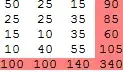
x = {{50, 25, 15}, {25, 25, 35}, {15, 10, 35}, {10, 40, 55}};

chisqt[x, "table"] yields:

chisqt[x, "expectedtable"] yields:

chisqt[x, "result"] yields:

chisqt[x, "fullresults"] yields:

chisqt[x, "Properties"] yields:

{"ChiSquareStatistic","p-value", "result", "table", "expectedtable", "fullresults"}