Piecewise Polynomial Interpolation

Question

Given some data pairs $(x_i,y_i)$, with $i=0,...,m$, and a degree $r$, I wish to build a piecewise polynomial function to interpolate these data. That interpolation should be continuous, and, on every interval $[x_k,x_{k+r}]$, with $k=0, r, 2r, ...$, should be a polynomial of degree $r$. This can be useful for example to represent the solution of a PDE obtained with finite element method of degree $r$.

Because with $r=1$ there are no problem I'll refer to $r=2$. For example, given the following data pairs:

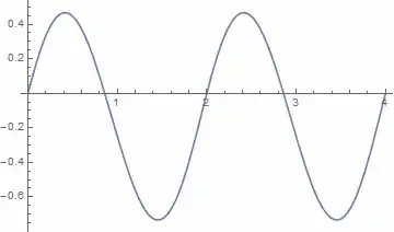
$$ \{ (0,0), (1,1), (2,0), (3,1), (4,0) \} $$

I wish to get this result:

The resulting interpolation function need not to have continuous derivative at $x=2$.

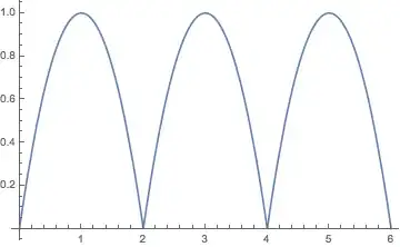
I tried with Interpolation and various options:

Interpolation[{{0, 0}, {1, 1}, {2, 0}, {3, 1}, {4, 0}}, 
 InterpolationOrder -> 2, Method -> "Hermite"]
Plot[%[x], {x, 0, 4}]

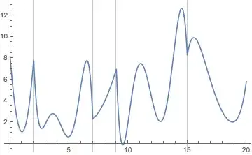
Interpolation[{{0, 0}, {1, 1}, {2, 0}, {3, 1}, {4, 0}}, 
 InterpolationOrder -> 2, Method -> "Spline"]
Plot[%[x], {x, 0, 4}]

As a reference, under MATLAB, I can build a piecewise polynomial interpolation of arbitrary degree, in a some involved way, with mkpp, and later consume the interpolation with ppval. For piecewise linear interpolation there is a more simple and direct interp1 function.

Under MATLAB I give to mkpp the values of the polinomials and their derivatives at $x_0, x_r, x_{2r}, ...$ and I get the expected result. Under Mathematica this approach doesn't work:

Interpolation[{{{0}, 0, 2, -2}, {{2}, 0, 2, -2}, {{4}, 0, 2, -2}}, 
 InterpolationOrder -> 2, Method -> "Hermite"]
Plot[%[x], {x, 0, 4}]

I considered using Piecewise and constructiong an Interpolation or a polynomial pure function for every interval $[x_k,x_{k+r}]$ but I suspect this become unmanageably complex when there are hundred or thousand of intervals.

There is some builtin way, reasonably simple and fast, to get this result? Naturally I search a general way, for general data and general $r$.

UPDATE

@kguler answer is interesting but I need a way to generalize for every $r$.

Answer 1

Based on What's inside InterpolatingFunction[{{1., 4.}}, <>]?, I would guess that a built-in way is not possible. However, one can take advantage of InterpolatingFunction to construct a Piecewise function. Here, split, does an overlapping partition starting a new list at position p, is a modification of Mr.Wizard's dPcore in this answer.

split[L_, pos_] := 
 Inner[L[[# - 1 ;; #2]] &, Prepend[pos + 1, 2], Append[pos, Length[L]], Head@L]

pwpolyifn[pts_, breaks_] := Function[x,
  Evaluate@
   Piecewise[{Interpolation[#, InterpolationOrder -> All][
        x], #[[1, 1]] <= x <= #[[-1, 1]]} & /@ split[pts, breaks]
    ]]

Example: split can do a ragged split.

split[{{0, 0}, {1, 1}, {2, 0}, {3, 1}, {4, 0}, {5, 1}, {6, 0}}, {3, 6}]
(*
  {{{0, 0}, {1, 1}, {2, 0}},
   {{2, 0}, {3, 1}, {4, 0}, {5, 1}},
   {{5, 1}, {6, 0}}}
*)

In this one, the OP's example, split[.., {3, 5}] is the same as Partition[.., 3, 2]:

split[{{0, 0}, {1, 1}, {2, 0}, {3, 1}, {4, 0}, {5, 1}, {6, 0}}, {3, 5}]
(*
  {{{0, 0}, {1, 1}, {2, 0}},
   {{2, 0}, {3, 1}, {4, 0}},
   {{4, 0}, {5, 1}, {6, 0}}}
*)

pwpolyifn[{{0, 0}, {1, 1}, {2, 0}, {3, 1}, {4, 0}, {5, 1}, {6, 0}}, {3, 5}][x]

Plot[pwpolyifn[{{0, 0}, {1, 1}, {2, 0}, {3, 1}, {4, 0}, {5, 1}, {6, 0}}, {3, 5}][x],
    {x, 0, 6}]

Another example:

SeedRandom[1];
pts = Table[{i, RandomReal[{0, 10}]}, {i, 0, 20}];
breaks = {3, 8, 10, 16};
Plot[Evaluate@pwpolyifn[pts, breaks][x], {x, 0, 20}, 
 GridLines -> {pts[[breaks]][[All, 1]], None}]

If bullet-proofing the definition is desired, then one can check that pts is a list of pairs of numbers and that the breaks are increasing and lie between 2 and Length[pts] - 1.

Answer 2

At present I'm still unable to find a builtin way to do this, so I decided to write my implementation just to go on.

A set of definitions to build the polinomial coefficients are needed. The first return a function to build the coefficients for degree $r$ and grid spacing $h=1$ and remember the result. The second is for generic $h$. The third accepts also function values and returns the coefficients instead of a function to build coefficients.

PiecewisePolynomialCoefficients[r_Integer /; r >= 1] := 
 PiecewisePolynomialCoefficients[r] =
  Evaluate[
    Block[{x}, 
     Reverse@CoefficientList[
        InterpolatingPolynomial[Table[{i, Slot[i + 1]}, {i, 0, r}], 
         x], x] // Simplify]] &
PiecewisePolynomialCoefficients[r_Integer /; r >= 1, h_] :=
 Evaluate[
   PiecewisePolynomialCoefficients[r] @@ Array[Slot, {r + 1}]/
    Table[h^i, {i, r, 0, -1}]] &
PiecewisePolynomialCoefficients[r_Integer /; r >= 1, h_, 
  yv_?VectorQ] := 
 PiecewisePolynomialCoefficients[r, h] @@ yv /; Length[yv] == r + 1

The coefficients are returned from the highest order to lowest so the following function can be used to evaluate the polinomial.

PolynomialHornerEvaluation[coeffs_?VectorQ, x_] := 
 Fold[(#1 x + #2) &, 0, coeffs]

The following function do the interpolation, compute polynomial coefficients and store info in a PiecewisePolynomialInterpolatingFunction object for later evaluation.

Options[PiecewisePolynomialInterpolation] := {InterpolationOrder -> 1};
PiecewisePolynomialInterpolation[
  xd : {xl_, xr_} /; NumericQ[xl] && NumericQ[xr] && xl < xr,
  yv_ /; VectorQ[yv] && Length[yv] >= 2,
  OptionsPattern[]] :=
 Module[{r, n, h, breaks, coeffs},
  r = OptionValue[InterpolationOrder];
  n = Length[yv];
  h = (xr - xl)/(n - 1);
  breaks = Range[xl, xr, r h];
  coeffs = 
   PiecewisePolynomialCoefficients[r, h] @@@ Partition[yv, r + 1, r];
  PiecewisePolynomialInterpolatingFunction[breaks, coeffs]
  ]

The following function dipslay relevant info of the PiecewisePolynomialInterpolatingFunction object.

MakeBoxes[
   PiecewisePolynomialInterpolatingFunction[breaks : {___}, 
    coeffs : {___}], form_] :=
  With[{dom = ToBoxes@Through[{First, Last}[breaks]], 
    order = ToBoxes[Length@First@coeffs - 1], 
    nodes = ToBoxes@Length[breaks]},
      RowBox[{"PiecewisePolynomialInterpolatingFunction[", 
     StyleBox[FrameBox[GridBox[
        {{"Domain:", dom}, {"Order:", order}, {"Nodes:", nodes}}]], 
      "DialogStyle", Gray, Small], "]"}]
      ];

The following definition evaluate the PiecewisePolynomialInterpolatingFunction object at some specific point $x$.

Needs["Combinatorica`"] (* For BinarySearch *)

PiecewisePolynomialInterpolatingFunction[breaks : {___}, 
   coeffs : {___}][x_?NumericQ] :=
  With[{i = Which[
     x < breaks[[1]], Message[InterpolatingFunction::dmval, x]; 1,
     x > breaks[[-1]], Message[InterpolatingFunction::dmval, x]; 
     Length[coeffs] - 1,
     True, Floor@BinarySearch[breaks, x]
     ]},
  PolynomialHornerEvaluation[coeffs[[i]], x - breaks[[i]]]
    ]

This way apparently works:

Any fix to this implementation (faster, safer, more generic) is appreciated. Any builtin solution also.

Answer 3

Perhaps too specific to OP's example case:

Interpolation[{{{0}, 0, Automatic}, {{1}, 1, 0}, {{2}, 0,  Automatic}, 
               {{3}, 1, 0}, {{4}, 0. Automatic}}, 
  InterpolationOrder -> 2]
  Plot[%[x], {x, 0, 4}]

and

 Interpolation[{{{0}, 0, Automatic}, {{1}, 1, 0}, {{2}, 0,  Automatic}, 
                {{3}, 1, 0}, {{4}, 0. Automatic}}, 
    InterpolationOrder -> 2, PeriodicInterpolation -> True]
 Plot[%[x], {x, 0, 8}]