the winding number for the circle map (Arnold tongue)

Question

I want to perform an iterative calculation and visualize the results:

f[n_, a_, b_] := Nest[# + a - b Sin[2 π #] &, 0, n]/n;

If I use machine precision, it probably results in greater error, for example:

N@f[500, 1/2, 3/5]
f[500, 0.5, 0.6]

(* 0.5 *)
(* 0.0282658 *)

Most of the time we can't use infinite precision and have to resort to using N.

How can I increase the accuracy of the results?

In addition, the iterative calculation is already quite slow, so it is also important to think about the efficiency of the solution.

I got started on this question while trying to explore properties of Circle Maps, and I would like to reproduce this image from the link:

My initial attempt looks like this:

f = Compile[{n, a, k}, Nest[# + a - k Sin[2 \[Pi] #] &, 0, n]/n];
dat =Outer[f[500, #2, #] &, Range[0, 1, 1/500], Range[0, 1, 1/500]]; // AbsoluteTiming
ArrayPlot[dat, 
   ColorFunction -> (Blend[{Black, Blue, Green, Yellow, Red}, #] &), 
   ColorFunctionScaling -> False, DataReversed -> True]

Which gives the following (unsatisfactory) result:

Answer 1

I have figured out why you are getting the structure you are getting. The reason has to do with your initial choice of the angle, which you set at $0$ in the Nest[] statement. The actual image is generated by choosing the mean result of iterating the map for many initial values chosen uniformly at random in $[0,1]$.

With $n = 50$ iterations and $m = 20$ trials, I obtained the following image using the following modification of your code:

f = Compile[{n, m, a, k}, Mean[Table[Nest[# + a - k Sin[2 Pi #] &,
    RandomReal[], n]/n, {j, 1, m}]]];
dat = Parallelize[Outer[f[50, 20, #2, #] &, Range[0, 1, 1/1000], 
    Range[0, 1, 1/1000]]];

I believe this is very, very close to exactly what you are looking for.

Answer 2

This question looks as a duplicate of these questions:

How to create internally optimized expression for computing with high WorkingPrecision?

How to work with Experimental`NumericalFunction?

An internally optimized version of the original function can be created as follows:

n = 500;
f = Experimental`CreateNumericalFunction[{a, b}, 
   Unevaluated[Nest[# + a - b Sin[2 \[Pi] #] &, 0, n]/n], {}, 
   WorkingPrecision -> 880];

How the created Experimental`NumericalFunction should be used:

f[{1/10, 1/5}]

0.00016666666666666666666666666666666666666666666666666666666666666666\
6666666666666666666666666666666666666666666666666666666666666666666666\
6666666666666666666666666666666666666666666666666666666666666666666666\
6666666666666666666666666666666666666666666666666666666666666666666666\
6666666666666666666666666666666666666666666666666666666666666666666666\
6666666666666666666666666666666666666666666666666666666666666666666666\
6666666666666666666666666666666666666666666666666666666666666666666666\
6666666666666666666666666666666666666666664685468521373229053036940442\
3962701216291153088605786704858607575162427563183707930229553541195321\
2101361759645135515775432980342040381738861309064752553797366691813555\
0017169360630698662587053257997111846801265386183928858616194265489581\
2949120884649269257779567658163657155358878262590630724222855526137604\
688700110160340115203634767418946813394731969

Here is a comparison of performance (updated):

<< GeneralUtilities`
ff[a_, b_] := Nest[# + a - b Sin[2 \[Pi] #] &, 0, n]/n;
o1 = ff[1/100, 1/500]; // AccurateTiming
o2 = ff[0.01`880, 1/500]; // AccurateTiming
o3 = f[{1/100, 1/500}]; // AccurateTiming

3.603673
0.0668274
0.068519

o2 == o3

True

As one can see from the timings, unfortunately in this concrete case Experimental`NumericalFunction does not increase performance as compared to the inexact case (o2) based on pure Nest.

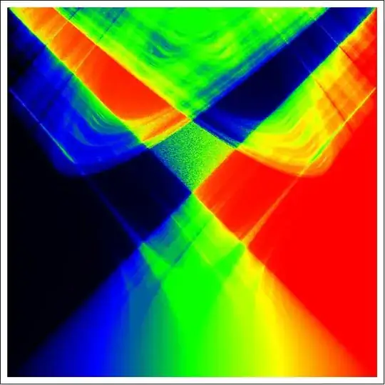
It means that the only way to increase performance of computing the ArrayPlot is to use parallelization. According to the documentation, "Outer products automatically parallelize" by Parallelize so the code in the question can be modified in straightforward way:

dat = Parallelize[Outer[f[500, #2, #] &, Range[0, 1.`880, 1/500], Range[0, 1.`880, 1/500]]]; // AbsoluteTiming
ArrayPlot[dat, 
   ColorFunction -> (Blend[{Black, Blue, Green, Yellow, Red}, #] &), 
   ColorFunctionScaling -> False, DataReversed -> True]

---

But even without parallelization it is possible to plot the problematic region in a reasonable time with precision 100 (MMa 8.0.4):

f[n_, a_, b_] := Nest[# + a - b Sin[2 \[Pi] #] &, 0, n]/n;

n = 500; prec = 100;
dat = Outer[f[n, #2, #] &, N[Range[4/10, 85/100, 1/n], prec], 
    N[Range[3/10, 7/10, 1/n], prec]]; // AbsoluteTiming
ArrayPlot[dat, 
 ColorFunction -> (Blend[{Black, Blue, Green, Yellow, Red}, #] &), 
 ColorFunctionScaling -> False, DataReversed -> True]

{501.2916722, Null}

And here is the result with prec = 300:

{1109.0984368, Null}

Answer 3

Incidentally, here is a higher resolution picture of the image produced by heropup's answer, plotted over both positive and negative values of the two circle map parameters:

Blue represents negative, yellow represents positive.

You can view a far larger 6001x6001 pixel image (about 29MB) here.

Here is the code used to generate the upper right quarter of the image (execution time with a 4-core i5-3550 was around 90 minutes):

f = Compile[{{a, _Real}, {k, _Real}}, 
   Mean[Table[
     Nest[# + a - k Sin[2 Pi #] &, j/1600 + RandomReal[{-1, 1}/6400], 
       50]/50, {j, 1600}]], CompilationTarget -> "C", 
   RuntimeAttributes -> {Listable}];
{tim, dat} = 
  AbsoluteTiming[
   Parallelize[
    Outer[f[#2, #] &, N@Range[0, 3, 1/1000], N@Range[0, 3, 1/1000]]]];
Export["ArnoldTongue.h5", dat]

Instead of averaging over random seed values between 0 and 1, this averages uniformly over the interval $[0,1]$ with a slight random noise added in; this accelerates the convergence to a smooth final image as compared to using random seeds, and thus reduces compute time.

The other 3/4 of the image can then be recovered by symmetry and antisymmetry. The resulting data was colored and rendered in Julia.

Answer 4

not an answer, just a cool animation:

Looping over the initial seed values from 0-1