4

I want to plot a function of 2 variables x and y, for discrete values of y, like:

myFunc[x_, y_] := Sin[x y]
yvalues={0.1,0.5,1.0,2.0}
Plot[Evaluate@Map[myFunc[x, #] &, yvalues], {x, 0, 5}]

What I want is that the maximum x range (in this case 5) is a function of yvalues, for example, for each value i of yvalues, stop the corresponding plot curve at Cos[yvalues[[i]]].

I need this because in my real case, the function to plot is a 2D interpolation which behaves badly outside some specific intervals depending on y.

Thanks.

Santiago
  • 1,201
  • 8
  • 16
  • You can add any of If, Piecewise, Boole and more to your definition of myFunc. – b.gates.you.know.what Aug 19 '14 at 09:46
  • @b.gatessucks thanks, but it is not possible, since in real life, myFunc is an interpolation function – Santiago Aug 19 '14 at 09:47
  • It should be related to something like this answer http://mathematica.stackexchange.com/a/20719/6138 – Santiago Aug 19 '14 at 09:51
  • Can't you do simply a table? Table[Plot[Sin[x i], {x, 0, i}], {i, 1, 5}] // Show[#, PlotRange -> All] & – chris Aug 19 '14 at 10:10
  • otherwise something like this? tt = {Sin[x], Cos[x], Cos[2 x]}; gg = {{0, 1}, {0, 2}, {0, 3}}; MapThread[Plot[#1, Evaluate@{x, Sequence @@ #2}] &, {tt, gg}]//Show – chris Aug 19 '14 at 10:13
  • or gg = {Table[{x, Sin[x]}, {x, 0, 10}] // Interpolation, Table[{x, Cos[x]}, {x, 0, 20}] // Interpolation}; Plot[#[x], {x, #[[1, 1, 1]], #[[1, 1, 2]]}] & /@ gg // Show – chris Aug 19 '14 at 10:15
  • @chris maybe it works, let me check. Anyway with your little example I get the same color for each curve, even if I use Evaluated->True or Evaluate – Santiago Aug 19 '14 at 10:26
  • then this Table[Plot[Sin[x i], {x, 0, 5 + i}, PlotStyle -> ColorData[10][i]], {i, 1, 3}] // Show[#, PlotRange -> All] & which is basically the same as eldo – chris Aug 19 '14 at 10:53

4 Answers4

5

A method using a single Plot expression:

myFunc[x_, y_] := Sin[x y]
yvalues = {0.1, 0.5, 1.0, 2.0, 3.0};

Block[{x},
 Plot[#, {x, -5, 5}, PlotRange -> All, PlotLegends -> Automatic] &[
  If[Cos[#] <= x <= 0 || 0 <= x <= Cos[#], myFunc[x, #]] & /@ yvalues
 ]
]

enter image description here

Notes:

  • I use Block to keep x localized.

  • I did not programmatically determine the range of the plot; I merely used -5, 5 and let PlotRange -> All clip the result. It would be better (but less clean) to determine the bounds from yvalues. I did not because I did not want to obscure this method. If desired I can add that however.

Mr.Wizard
  • 271,378
  • 34
  • 587
  • 1,371
  • thanks, looks good and the clipping with PlotRange would suit my needs I think. If you want you can post the better method, so I can learn something. – Santiago Aug 19 '14 at 21:50
  • @Santi You're welcome. kguler already posted the calculated bounds method in his answer so I won't duplicate that. – Mr.Wizard Aug 19 '14 at 21:53
5

Another method with a single plot:

ClearAll[myFunc2];
yvalues = {0.1`, 0.5`, 1.`, 2.`, 3.`};

myFunc2[x_?NumericQ, y_?NumericQ] := 
       ConditionalExpression[Sin[x y], IntervalMemberQ[Interval[{0, Cos[y]}], x]];
{min, max} = Through[{Min, Max}[Cos[yvalues]]];

Plot[myFunc2[x, #] & /@ yvalues, {x, min, max}, Evaluated -> True, BaseStyle -> Thick,
       ImageSize -> 600,  PlotLegends -> "Expressions"] /. myFunc2[a_, b_] :> Sin[ a b]

enter image description here

Edit: Another alternative is to use

myFunc3[x_, y_] :=  ConditionalExpression[Sin[x y], Min[0, Cos[y]] <= x <= Max[0, Cos[y]]];

instead of myFunc2.

kglr
  • 394,356
  • 18
  • 477
  • 896
  • thanks, that's a nice solution. I still have to understand how this thing with ConditionalExpression and IntervalMemberQ work. – Santiago Aug 19 '14 at 21:51
  • 1
    @Santi This is pretty much what I did but using alternative functions. I chose If because it's terse and as just about everyone here knows I like that. IntervalMemberQ takes the place of Cos[#] <= x <= 0 || 0 <= x <= Cos[#] in mine. – Mr.Wizard Aug 19 '14 at 21:56
3

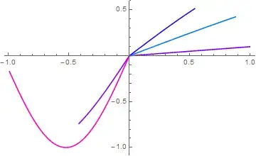
Is something like this your intention?

myFunc[x_, y_] := Sin[x y]

yvalues = {0.1, 0.5, 1.0, 2.0, 3.0};

fun = Map[myFunc[x, #] &, yvalues];

lim = Table[Cos[yvalues[[i]]], {i, 1, 5}];

plot =
 Table[Plot[fun[[j]], {x, 0, lim[[j]]},
   PlotStyle -> {Red, Green, Blue, Orange, Brown}[[j]]], {j, 1, 5}]

Show[plot, PlotRange -> All]

enter image description here

eldo
  • 67,911
  • 5
  • 60
  • 168
  • yes thanks! I think that would do it. I never thought of using Show, I supposed there was a way to do it inside one single Plot, but this works for me! – Santiago Aug 19 '14 at 10:28
3

If eldo's plot is your desired outcome you could also do:

Show[Plot[Sin[x #], {x, 0, Cos@#}, PlotStyle -> Hue[RandomReal[]]] & /@
   yvalues, PlotRange-> All]

enter image description here

Noting Cos2 and Cos[3] are negative.

If you want legends:

With[{col = Hue /@ RandomReal[{0, 1}, 5]},
 Legended[
  Show[MapThread[
    Plot[Sin[x #1], {x, 0, Cos@#1}, PlotStyle -> #2] &, {yvalues, 
     col}], PlotRange -> All], 
  LineLegend[col, Sin[# x] & /@ yvalues]]]

enter image description here

ubpdqn
  • 60,617
  • 3
  • 59
  • 148