Speed up Schwarz-Christoffel mapping

Question

I would like to ask your advice how to speed up Contour and Parametric plots in the following example.

Let as start by defining a function

A = {(8 Sqrt[1035741])/15625, 0, 0, 0, 0, Sqrt[6597877/15]/6250, 0, 0, 0, 
0, -(Sqrt[(6338501/10)]/3125), 0, 0, 0, 0, (29 Sqrt[27347/30])/3125, 0, 0, 
0, 0, -(Sqrt[(4358874/5)]/3125), 0, 0, 0, 0, -(Sqrt[(352454081/3)]/31250), 
0, 0, 0};
Clear[s]
s[m_, l_] := If[m < 0, (-1)^m s[-m, l]]
s[m_?NonNegative, l_] := If[Abs[m] <= l, A[[m + 1]], 0]
Clear[ysaf]
L = 28;
ysaf[θ_, ϕ_] = 
ExpToTrig[Sum[s[m, L] SphericalHarmonicY[L, m, θ, ϕ], {m, -5 IntegerPart[L/5], L, 5}]];

ysaf is a pretty complicated trigonometric function of two angles in spherical coordinate system.

Next, we define a few parameters for a stereographic projection. I am plotting a part of the unit sphere as seen from a point on z-axis.

θmx = ArcCos[1/Sqrt[5]];
λ = 3/4;
rmx = Sin[θmx/λ];

Following plot takes a minute or so

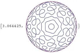
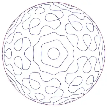
gr = ContourPlot[{ysaf[λ ArcSin[Sqrt[x^2 + y^2]] , ArcTan[x, y]] == 0,
Sqrt[x^2 + y^2] == rmx}, {x, -rmx, rmx}, {y, -rmx, rmx}, 
RegionFunction -> Function[{x, y, z}, Sqrt[x^2 + y^2] <= rmx], 
Axes -> False, Frame -> False]

Next, I am constructing interpolating functions for contour lines (like in this post)

lines = Cases[Normal[gr], Line[i__] -> i, Infinity];
fns = Map[Map[ListInterpolation[#, {{0, 1}}] &, Transpose[#]] &, lines];

and define a Schwarz-Christoffel map (see p. 468 of Complex Analysis with MATHEMATICA® by W. T. Shaw, isbn 0521836263):

PolyMap[z_] = Integrate[1/(1 - ξ^5)^(2/5), {ξ, 0, z}];

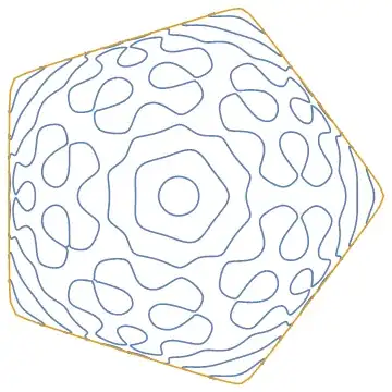
This final plot is the objective of my question. How can I speed it up?

ParametricPlot[
Table[PolyMap[(Through[fns[[a]][x]]/rmx) /. {List -> Complex}] /. 
Complex[i_, j_] :> {i, j}, {a, 1, First[Dimensions[fns]]}], {x, 0, 1}, Axes -> False, Frame -> False]

plot1

plot2

Any help is appreciated!

Extremely nice plots. Despite some efforts I couldn't make them faster. Will try tomorrow again. — eldo, Aug 29 '14 at 22:05

score 5 · Accepted Answer · answered Aug 30 '14 at 11:00

You can get a significant boost by compiling ysaf:

ysafc = Compile[{x, y}, Evaluate @ N @ ysaf[λ ArcSin[Sqrt[x^2 + y^2]], ArcTan[x, y]]];

func[x_?NumericQ, y_?NumericQ] := ysafc[x, y]

gr = ContourPlot[{func[x, y] == 0, Sqrt[x^2 + y^2] == rmx}, {x, -rmx, rmx}, {y, -rmx, rmx}, 
  RegionFunction -> Function[{x, y, z}, Sqrt[x^2 + y^2] <= rmx], 
  Axes -> False, Frame -> False]

For the mapping I would suggest transforming the coordinate data in gr directly. I have also used GenerateConditions -> False in the integral to remove the ConditionalExpression:

PolyMap[z_] = Integrate[1/(1 - ξ^5)^(2/5), {ξ, 0, z}, GenerateConditions -> False];

pm[{x_, y_}] := Through[{Re, Im} @ PolyMap[x + I y]]

Show[Normal[gr] /. Line[data_] :> Line[pm /@ data], PlotRange -> All]

enter image description here

I learnt a lot from your answer. Even though your code was not the fastest for the ContourPlot I am accepting this answer because it gives an incredible boost was the second part -the Schwarz-Cristoffel transform. This was the slowest part of the code and now it runs in less than 1 sec! — yarchik, Sep 01 '14 at 08:11
Even easier: PolyMap[z_] = Integrate[1/(1 - z^5)^(2/5), z]. — J. M.'s missing motivation, Oct 18 '15 at 19:00

PhilChang · Answer 2 · 2014-08-30T11:48:54.183

The orginal program takes 78s on my computer. First, Make vector A a real vector will make the program a little faster.

 A = {(8 Sqrt[1035741])/15625, 0, 0, 0, 0, Sqrt[6597877/15]/6250, 0, 0,
     0, 0, -(Sqrt[(6338501/10)]/3125), 0, 0, 0, 
    0, (29 Sqrt[27347/30])/3125, 0, 0, 0, 
    0, -(Sqrt[(4358874/5)]/3125), 0, 0, 0, 
    0, -(Sqrt[(352454081/3)]/31250), 0, 0, 0} // N;

Second, avoiding recursive in function s also help.

s[m_, l_] := If[Abs[m] > l, 0,
    If[Negative[m], (-1)^m A[[(-m) + 1]], A[[m + 1]] ]

Third, Sum is a little bit slow. Use Dot instead. And ExpToTrig is not necessary.

mlist = Table[m, {m, -5 IntegerPart[L/5], L, 5}];
ysaf[θ_, ϕ_] = 

   Dot[s[#, L] & /@ mlist, 
    SphericalHarmonicY[L, #, θ, ϕ] & /@ mlist];

Fourth,Evaluate

gr = ContourPlot[
  Evaluate@{  
    ysaf[λ ArcSin[Sqrt[x^2 + y^2]], ArcTan[x, y]] == 0.0, 
    Sqrt[x^2 + y^2] == rmx}, {x, -rmx, rmx}, {y, -rmx, rmx}, 
  RegionFunction -> Function[{x, y, z}, Sqrt[x^2 + y^2] <= rmx], 
  Axes -> False, Frame -> False]

In this way, the contour plot gr cost 20s compared with original 78s on my computer.

Besides, if you define your function ysaf as

ysafNew[x_, y_] := 
 With[{  θ = λ ArcSin[Sqrt[x^2 + y^2]], ϕ = 
    ArcTan[x, y]},
                Re@Dot[slist, SphericalHarmonicY[L, mlist, θ, ϕ]]

the time will be 9s.

I hope someone could improve more.

In ParametricPlot, Use MaxRecursion and Plotpoints

ParametricPlot[
Table[PolyMap[(Through[fns[[a]][x]]/rmx) /. {List -> Complex}] /. 
Complex[i_, j_] :> {i, j}, {a, 1, First[Dimensions[fns]]}],
{x, 0, 1}, Axes -> False, Frame -> False, 
MaxRecursion -> 2, 
PlotPoints -> 30]

============================================================================================== Here is all the code:

    Remove["Global`*"];
A = {(8 Sqrt[1035741])/15625, 0, 0, 0, 0, Sqrt[6597877/15]/6250, 0, 0,
     0, 0, -(Sqrt[(6338501/10)]/3125), 0, 0, 0, 
    0, (29 Sqrt[27347/30])/3125, 0, 0, 0, 
    0, -(Sqrt[(4358874/5)]/3125), 0, 0, 0, 
    0, -(Sqrt[(352454081/3)]/31250), 0, 0, 0} // N;
Clear[s]
(*s[m_,l_]:=If[m<0,(-1)^m s[-m,l]]
s[m_?NonNegative,l_]:=If[Abs[m]≤l,A[[m+1]],0]*)
s[m_, l_] := If[Abs[m] > l, 0,
    If[Negative[m], (-1)^m A[[(-m) + 1]], A[[m + 1]] ]
  ]
Clear[ysaf]
L = 28;
(*ysaf[θ_,ϕ_]=ExpToTrig[Sum[s[m,L] \
SphericalHarmonicY[L,m,θ,ϕ],{m,-5 \
IntegerPart[L/5],L,5}]];*)
mlist = Table[m, {m, -5 IntegerPart[L/5], L, 5}];
slist = s[#, L] & /@ mlist; 
ysaf[θ_, ϕ_] = 
  Dot[s[#, L] & /@ mlist, 
   SphericalHarmonicY[L, mlist, θ, ϕ]] ;
θmx = ArcCos[1.0/Sqrt[5.0]];
λ = 3.0/4.0;
rmx = Sin[θmx/λ];
ysafNew[x_, y_] := 
  With[{  θ = λ ArcSin[Sqrt[x^2 + y^2]], ϕ = 
     ArcTan[x, y]},
                Re@Dot[slist, SphericalHarmonicY[L, mlist, θ, ϕ]]
        ];
{time, gr} = 
 ContourPlot[
   Evaluate@{ysafNew[x, y] == 0.0, Sqrt[x^2 + y^2] == rmx}, {x, -rmx, 
    rmx}, {y, -rmx, rmx}, 
   RegionFunction -> Function[{x, y, z}, Sqrt[x^2 + y^2] <= rmx], 
   Axes -> False, Frame -> False] // AbsoluteTiming

enter image description here

Aside from the fact that your answer contains several typos I cannot confirm at all your timings. Any proof? — eldo, Aug 30 '14 at 08:20
@eldo, I pasted all my source code in my answer, if you can not run the code, please let me know. I did not understand how to get fns and the function inside the ParametricPlot very much, so I can not optimize the performance. — PhilChang, Aug 30 '14 at 08:47

score 4 · Answer 3 · edited Aug 30 '14 at 10:55

Some codes are from the answer of PhilChang

Remove["Global`*"];
A = {(8 Sqrt[1035741])/15625, 0, 0, 0, 0, Sqrt[6597877/15]/6250, 0, 0,
     0, 0, -(Sqrt[(6338501/10)]/3125), 0, 0, 0, 0, (29 Sqrt[27347/30])/3125, 0, 0, 0, 
    0, -(Sqrt[(4358874/5)]/3125), 0, 0, 0, 0, -(Sqrt[(352454081/3)]/31250), 0, 0, 0} // N;
s[m_, l_] := If[Abs[m] > l, 0, If[Negative[m], (-1)^m A[[(-m) + 1]], A[[m + 1]]]]
L = 28;
mlist = Table[m, {m, -5 IntegerPart[L/5], L, 5}];
slist = s[#, L] & /@ mlist;
ysaf[θ_, ϕ_] = Dot[s[#, L] & /@ mlist, SphericalHarmonicY[L, mlist, θ, ϕ]];
θmx = ArcCos[1.0/Sqrt[5.0]];
λ = 3.0/4.0;
rmx = Sin[θmx/λ];

ysafNew = 
 Compile[{{x, _Real}, {y, _Real}}, 
  Evaluate@With[{θ = λ ArcSin[
        Sqrt[x^2 + y^2]], ϕ = ArcTan[x, y]}, 
    Re@Dot[slist, SphericalHarmonicY[L, mlist, θ, ϕ]]]];

ContourPlot[{ysafNew[x, y] == 0.0, Sqrt[x^2 + y^2] == rmx}, {x, -rmx, 
    rmx}, {y, -rmx, rmx}, 
   RegionFunction -> Function[{x, y, z}, Sqrt[x^2 + y^2] <= rmx], 
   Axes -> False, Frame -> False] // Quiet // AbsoluteTiming

Mathematica graphics

hi,do you know how to optimize fns and ParametricPlot? i can not understand what it means — PhilChang, Aug 30 '14 at 09:45
@ Chenminqi When I tried your solution on my machine I got incredible 1.4 sec! Combining your answer with the solution of @Simon Woods for the Schwarz-Cristoffel mapping I am getting 1.4 + 0.8 sec in total! — yarchik, Sep 01 '14 at 08:20

eldo · Answer 4 · 2014-08-30T11:20:01.023

One can gain a considerable speed gain by omitting RegionFunction and setting PlotPoints to 10. The following only needs 8 seconds (it uses some ideas of @PhilChang):

A = {
   (8 Sqrt[1035741])/15625, 0, 0, 0, 0,
   Sqrt[6597877/15]/6250, 0, 0, 0, 0,
   -(Sqrt[(6338501/10)]/3125), 0, 0, 0, 0,
   (29 Sqrt[27347/30])/3125, 0, 0, 0, 0,
   -(Sqrt[(4358874/5)]/3125), 0, 0, 0, 0,
   -(Sqrt[(352454081/3)]/31250), 0, 0, 0
   };

s[m_, l_] := If[Abs[m] > l, 0, If[Negative[m], (-1)^m A[[(-m) + 1]], A[[m + 1]]]]

L = 16;
mx = ArcCos[1/Sqrt[5]];
lambda = 3/4;
rmx = Sin[mx/lambda];
mlist = Table[m, {m, -5 IntegerPart[L/5], L, 5}];
slist = s[#, L] & /@ mlist;
hlist = SphericalHarmonicY[L, #, a, b] & /@ mlist;

ysaf[a_, b_] = Dot[slist, hlist];

ContourPlot[
  ysaf[lambda ArcSin[Sqrt[x^2 + y^2]], ArcTan[x, y]],
  {x, -rmx, rmx}, {y, -rmx, rmx},
  ColorFunction -> "DarkRainbow",
  Contours -> 6,
  PlotPoints -> 10,
  PlotLegends -> Automatic]

enter image description here

Plot3D[
  ysaf[lambda ArcSin[Sqrt[x^2 + y^2]], ArcTan[x, y]],
  {x, -rmx, rmx}, {y, -rmx, rmx},
  ColorFunction -> "DarkRainbow",
  PlotPoints -> 50,
  ImageSize -> 500,
  PlotLegends -> Automatic]

enter image description here

Speed up Schwarz-Christoffel mapping

4 Answers4