Solving a two point boundary problem for a piecewise system of equations

Question

I'm trying to solve a two point boundary value problem with a piecewise system of equations like:

dx[t_] := Piecewise[{{0, y[t] <= 0}, {x[t]^(3/4) - x[t], y[t] > 0}}]
dy[t_] := Piecewise[{{0, y[t] <= 0}, {(1 - y[t])/x[t]^(1/4) + y[t], y[t] > 0}}]

NDSolve[{x'[t] == dx[t], y'[t] == dy[t], x[0] == 1, y[10] == 2}, {x, y}, {t, 0, 10}]

which produces the error

 NDSolve::bvdisc: NDSolve is not currently able to solve boundary value problems with discrete variables.

I tried the answers here by entering

funs = ParametricNDSolveValue[{x'[t] == dx[t], y'[t] == dy[t], x[0] == 1, y[10] == yt}, {x, y}, {t, 0, end}, yt]

FindRoot[funs[yt][end], {yt, 2}]

which yields the same error.

Is there any way to solve this system? Thanks for the help.

Answer 1

There is no need to use Piecewise because both $x(t)$ as well as $y(t)$ remain non negative. Furthermore, the equation for x is independent of y and can be solved analytically.

The result $x(t)$ is then put into the equation for $y(t)$ which will be solved numerically.

Finally we verify our first statement about the non-negativity.

Ok, here we go.

The eqution for $x(t)$ is

sx = DSolve[x'[t] == x[t]^(3/4) - x[t] && x[0] == 1, x[t], t]

We can safely ignore the error messages; they are just information which is not relevant here.

(* Out[105] = {{x[t] -> E^-t (-2 + E^(t/4))^4}, {x[t] -> E^-t ((-1 - I) + E^(t/4))^4}, {x[t] -> E^-t ((-1 + I) + E^(t/4))^4}} *)

Taking the real-valued solution

xx[t_] = x[t] /. sx[[1]]

(* Out[106]= E^-t (-2 + E^(t/4))^4 *)

Plot[xx[t], {t, 0, 30}]

Now solving numerically the equation for $y(t)$ using the previously obtained function $xx(t)$:

sy = NDSolve[y'[t] == (1 - y[t])/xx[t]^(1/4) + y[t] && y[0] == 10, y[t], {t, 0, 50}][[1]]

$\{y[t]\to \text{InterpolatingFunction}[\{\{0.,50.\}\},<>][t]\}$

Works out smoothly, no precision problems. Here's the function itself

yy[t_] = y[t] /. sy

$\text{InterpolatingFunction}[\{\{0.,50.\}\},<>][t]$

Finally ploting both functions together, magnifying $x(t)$ by a factor of ten for better visibility:

Plot[{10 xx[t], yy[t]}, {t, 0, 30}, PlotRange -> {-1, 20}, PlotLabel -> "blue x(t), red y(t)"]

Nice problem. Hope this helps.

Regards, Wolfgang

Answer 2

Here is now the - hopefully - correct (numeric) solution of the original problem.

To begin with, we define a time t0 such that y = 0 for 0<=t<=t0.

Für x(t) we have x(t) = 1 for 0<=t<=t0, otherwise we have first to solve the equation

sx = DSolve[x'[t] == x[t]^(3/4) - x[t] && x[0] == 1, x[t], t]

We can ignore the error Messages.

(* Out[701]= {{x[t] -> E^-t (-2 + E^(t/4))^4}, {x[t] -> 
   E^-t ((-1 - I) + E^(t/4))^4}, {x[t] -> E^-t ((-1 + I) + E^(t/4))^4}} *)

Taking the real-valued solution:

x[t] /. sx[[1]]

(* Out[700]= E^-t (-2 + E^(t/4))^4 *)

Having caluclated that, we now define the complete function x[t,t0]

x[t_, t0_] := E^(-t + t0) (-2 + E^((t - t0)/4))^4 /; t > t0

x[t_, t0_] := 1 /; 0 <= t <= t0

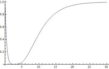
Plotting it (for t0 = 5)

Plot[{x[t, 5]}, {t, 0, 30}, PlotRange -> {0, 1}]

Now inserting x[t,t0] we can NDSolve for y(t). Here we have selected the parameter t0 by trial and error such that y[10]=2

t0 = 1.03214; 
ta = 0;
te = 12;
sn = NDSolve[{D[y[t], t] == 1 - y[t] (1/x[t, t0]^(1/4) - 1), y[t0] == 0}, 
    y[t], {t, ta, te}][[1]];
{ta, te} = Head[(List @@ sn[[1]])[[2]]][[1, 1]];
yy[t_] = y[t] /. sn;
Print["y[10] = ", yy[10]];
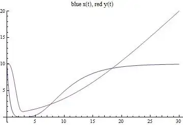
Plot[{2, Evaluate[x[t, t0]], yy[t]}, {t, ta, te}, PlotRange -> {-1, 2.2}, 
 PlotLabel -> 
  "Solution of the two-point boundary problem\nred curve = x(t), green curve \
= y(t)\nt0 = " <> ToString[t0] <> "\ty(10) = " <> ToString[yy[10]]]

y[10] = 2.

Of course, y(t) must be set to zero below t=t0. This is trivial and not shown in the picture.

This seems to be the only solution. For greater values of t0 the boundary value y(10) decreases, and for smaller it increases.

Regards, Wolfgang