(Very) ill-behaved Piecewise Plot

Question

I am interested in defining a function (with arguments: a symbol for a variable and a list of 6 points) that represents a quadratic interpolating spline of the points. Here is my attempt

f20[x_, P_, Q_, R_, S_, T_, U_] := 
  InterpolatingPolynomial[{{{P[[1]]}, P[[2]], 0}, {{Q[[1]]}, 
     Q[[2]]}}, {x}];
f21[x_, P_, Q_, R_, S_, T_, U_] := 
  InterpolatingPolynomial[{{{Q[[1]]}, Q[[2]], 
     D[f20[x, P, Q, R, S, T, U], x] /. x -> Q[[1]]}, {{R[[1]]}, 
     R[[2]]}}, {x}];
f22[x_, P_, Q_, R_, S_, T_, U_] := 
  InterpolatingPolynomial[{{{R[[1]]}, R[[2]], 
     D[f21[x, P, Q, R, S, T, U], x] /. x -> R[[1]]}, {{S[[1]]}, 
     S[[2]]}}, {x}];
f23[x_, P_, Q_, R_, S_, T_, U_] := 
  InterpolatingPolynomial[{{{S[[1]]}, S[[2]], 
     D[f22[x, P, Q, R, S, T, U], x] /. x -> S[[1]]}, {{T[[1]]}, 
     T[[2]]}}, {x}];
f24[x_, P_, Q_, R_, S_, T_, U_] := 
  InterpolatingPolynomial[{{{T[[1]]}, T[[2]], 
     D[f23[x, P, Q, R, S, T, U], x] /. x -> T[[1]]}, {{U[[1]]}, 
     U[[2]]}}, {x}];
Interp2[x_, P_, Q_, R_, S_, T_, U_] := 
  Piecewise[{{f20[x, P, Q, R, S, T, U], 
     P[[1]] <= x <= Q[[1]]}, {f21[x, P, Q, R, S, T, U], 
     Q[[1]] < x <= R[[1]]}, {f22[x, P, Q, R, S, T, U], 
     R[[1]] < x <= S[[1]]}, {f23[x, P, Q, R, S, T, U], 
     S[[1]] < x <= T[[1]]}, {f24[x, P, Q, R, S, T, U], 
     T[[1]] < x <= U[[1]]}}];

Then I try to evaluate the function and plot it

Interp2[s, {1, 1}, {2, 3}, {3, 3}, {4, 4}, {5, 5}, {6, 3}]
Plot[Interp2[s, {1, 1}, {2, 3}, {3, 3}, {4, 4}, {5, 5}, {6, 3}], {s, 
  1, 6}, PlotRange -> Full]

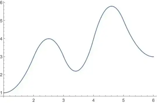
The output is the following (problem 1)

which seems very weird because the function is correct but the plot is not.

If I manually edit the first output to plot the function (with the same code as the second line of the input), or if I use the code

Interp2[s, {1, 1}, {2, 3}, {3, 3}, {4, 4}, {5, 5}, {6, 3}]
Plot[%, {s, 1, 6}, PlotRange -> Full]

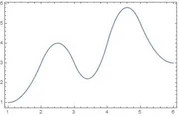
instead, I get this (problem 2)

Notably, the plot is discontinuous, but the discontinuity points are not always matching the extremal points of the intervals in the piecewise definition: the gap near s = 4 is between s = 4.1 and s = 4.2. In this second case, I tried various options of MaxRecursion and PerformanceGoal to obtain a better quality, with no different results as the one in the picture.

I am interested in a solution for problem 1 (rather than 2), but any suggestion is very welcome.

Thanks

Answer 1

Attributes[Plot]

{HoldAll, Protected, ReadProtected}

Since Plot has attribute HoldAll, you need to use Evaluate. Also, use of Exclusions at transition values avoids gaps in the Plot:

f20[x_, P_, Q_, R_, S_, T_, U_] :=
  InterpolatingPolynomial[
   {{{P[[1]]}, P[[2]], 0}, {{Q[[1]]}, Q[[2]]}},
   {x}];
f21[x_, P_, Q_, R_, S_, T_, U_] :=
  InterpolatingPolynomial[
   {{{Q[[1]]}, Q[[2]], 
     D[f20[x, P, Q, R, S, T, U], x] /.
      x -> Q[[1]]}, {{R[[1]]}, 
     R[[2]]}}, {x}];
f22[x_, P_, Q_, R_, S_, T_, U_] :=
  InterpolatingPolynomial[
   {{{R[[1]]}, R[[2]], 
     D[f21[x, P, Q, R, S, T, U], x] /.
      x -> R[[1]]}, {{S[[1]]}, 
     S[[2]]}}, {x}];
f23[x_, P_, Q_, R_, S_, T_, U_] :=
  InterpolatingPolynomial[
   {{{S[[1]]}, S[[2]], 
     D[f22[x, P, Q, R, S, T, U], x] /.
      x -> S[[1]]}, {{T[[1]]}, 
     T[[2]]}}, {x}];
f24[x_, P_, Q_, R_, S_, T_, U_] :=
  InterpolatingPolynomial[
   {{{T[[1]]}, T[[2]], 
     D[f23[x, P, Q, R, S, T, U], x] /.
      x -> T[[1]]}, {{U[[1]]}, 
     U[[2]]}}, {x}];
Interp2[x_, P_, Q_, R_, S_, T_, U_] :=
  Piecewise[{
    {f20[x, P, Q, R, S, T, U], P[[1]] <= x <= Q[[1]]},
    {f21[x, P, Q, R, S, T, U], Q[[1]] < x <= R[[1]]},
    {f22[x, P, Q, R, S, T, U], R[[1]] < x <= S[[1]]},
    {f23[x, P, Q, R, S, T, U], S[[1]] < x <= T[[1]]},
    {f24[x, P, Q, R, S, T, U], T[[1]] < x <= U[[1]]}}];

Interp2[s, {1, 1}, {2, 3}, {3, 3}, {4, 4}, {5, 5}, {6, 3}]

Plot[
 Evaluate[
  Interp2[s, {1, 1}, {2, 3}, {3, 3}, {4, 4}, {5, 5}, {6, 3}]],
 {s, 1, 6},
 PlotRange -> Full,
 Exclusions -> Range[6]]

Answer 2

In fact, one can use Interpolation[] to build the required quadratic spline. Notice that in the constructed Interp2[], the slope at the right of one parabola is then fed into the parabola after that as its slope at the left (hence a spline). FoldList[] can be used to compact the code used by the OP:

pp = FoldList[Append[#2, D[InterpolatingPolynomial[{##}, \[FormalX]], \[FormalX]] /.
                         \[FormalX] -> #2[[1, 1]]] &,
              {{{1}, 1, 0}, {{2}, 3}, {{3}, 3}, {{4}, 4}, {{5}, 5}, {{6}, 3}}]
   {{{1}, 1, 0}, {{2}, 3, 4}, {{3}, 3, -4}, {{4}, 4, 6}, {{5}, 5, -4}, {{6}, 3, 0}}

ifun = Interpolation[pp, InterpolationOrder -> 2];

Plot[ifun[x], {x, 1, 6}]

You can check that this is equivalent to the Piecewise[] expression generated by Interp2[].